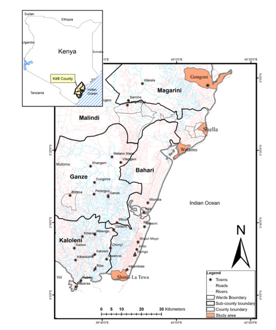
This paper examines the nexus between marine fishery dependence, poverty and inequality among households in coastal lowlands of Kenya, specifically, Kilifi County. Data for the study were collected from 384 randomly selected households through structured pretested questionnaires. The study used the multidimensional poverty methodology and multivalued treatment effect model to determine the marine fishery dependence of households, poverty, and inequality nexus. Findings from the study show that increasing ocean fishery dependence is associated with increased poverty and inequality among the dependent households. However, it is worth mentioning that other factors may as well affect poverty. Results also revealed that fishing was not a choice, but rather a necessity with approximately 71.3% of the dependent households reporting a lack of alternative livelihood options. More so, the dependent households that pursued diversification livelihood strategies had a lower deprivation score at 0.29 compared to 0.47 that engaged solely in fishing. Welfare policies such as the establishment of Beach Management Units (BMU), No Take Zones (NTZs), locally managed marine areas (LMMAs), and information networks have been put in place to promote the livelihoods of the fishing communities. However, their implementation has been ineffective leading to social exclusion and hence poverty traps among the poorest dependent households. The study, therefore, recommends strengthening existing governance options while putting a special focus on gear regulations.
Citation: Mohamed Idris Somoebwana, Oscar Ingasia Ayuya, John Momanyi Mironga. Marine fishery dependence, poverty and inequality nexus along the coastal lowlands of Kenya[J]. National Accounting Review, 2021, 3(2): 152-178. doi: 10.3934/NAR.2021008
This paper examines the nexus between marine fishery dependence, poverty and inequality among households in coastal lowlands of Kenya, specifically, Kilifi County. Data for the study were collected from 384 randomly selected households through structured pretested questionnaires. The study used the multidimensional poverty methodology and multivalued treatment effect model to determine the marine fishery dependence of households, poverty, and inequality nexus. Findings from the study show that increasing ocean fishery dependence is associated with increased poverty and inequality among the dependent households. However, it is worth mentioning that other factors may as well affect poverty. Results also revealed that fishing was not a choice, but rather a necessity with approximately 71.3% of the dependent households reporting a lack of alternative livelihood options. More so, the dependent households that pursued diversification livelihood strategies had a lower deprivation score at 0.29 compared to 0.47 that engaged solely in fishing. Welfare policies such as the establishment of Beach Management Units (BMU), No Take Zones (NTZs), locally managed marine areas (LMMAs), and information networks have been put in place to promote the livelihoods of the fishing communities. However, their implementation has been ineffective leading to social exclusion and hence poverty traps among the poorest dependent households. The study, therefore, recommends strengthening existing governance options while putting a special focus on gear regulations.

| [1] |
Akongyuure DN, Amisah S, Agyemang TK, et al. (2017) Tono reservoir fishery contribution to poverty reduction among fishers in Northern Ghana. Afr J Aquat Sci 42: 143-154. doi: 10.2989/16085914.2017.1344120

|
| [2] |
Alkire S, Foster J (2011) Counting and multidimensional poverty measurement. J Public Econ 95: 476-487. doi: 10.1016/j.jpubeco.2010.11.006
|
| [3] | Alkire S, Santos ME (2013) Measuring acute poverty in the developing world: robustness and scope of the multidimensional poverty index. OPHI Working Paper 59. Oxford: University of Oxford. |
| [4] | Alkire S, Suman S (2014) Inequality among the MPI poor, and regional disparity in multidimensional poverty: Levels and trends. OPHI Briefing 25. Oxford: University of Oxford. |
| [5] | Alkire S, Seth S (2014) Measuring and decomposing inequality among multidimensionally poor using ordinal data: a counting approach. OPHI Working Papers 68. Oxford: University of Oxford. |
| [6] | Angelsen A, Jagger P, Babigumira R, et al. (2014) Environmental income and rural livelihoods: a global-comparative analysis. World Dev 64: S12-S28. |
| [7] |
Ayuya OI, Gido EO, Bett HK, et al. (2015) Effect of certified organic production systems on poverty among smallholder farmers: empirical evidence from Kenya. World Dev 67: 27-37. doi: 10.1016/j.worlddev.2014.10.005
|
| [8] | Batista VS, Fabré NN, Malhado AC, et al. (2014) Tropical artisanal coastal fisheries: challenges and future directions. Rev Fish Sci 22: 1-15. |
| [9] |
Bavinck M, Jentoft S, Scholtens J (2018) Fisheries as social struggle: a reinvigorated social science research agenda. Mar Policy 94: 46-52. doi: 10.1016/j.marpol.2018.04.026
|
| [10] |
Beckline M, Yujun S, Etongo D, et al. (2018) Assessing the drivers of land use change in the rumpi hills forest protected area, Cameroon. J Sustain Forest 37: 592-618. doi: 10.1080/10549811.2018.1449121
|
| [11] |
Béné C, Friend RM (2011) Poverty in small-scale fisheries: old issue, new analysis. Prog Dev Stud 11: 119-144. doi: 10.1177/146499341001100203
|
| [12] |
Béné C, Arthur R, Norbury H, et al. (2016) Contribution of fisheries and aquaculture to food security and poverty reduction: assessing the current evidence. World Dev 79: 177-196. doi: 10.1016/j.worlddev.2015.11.007
|
| [13] |
Bia M, Mattei A (2008) A stata package for the estimation of the dose-response function through adjustment for the generalized propensity score. Stata J 8: 354-373. doi: 10.1177/1536867X0800800303
|
| [14] |
Bia M, Mattei A (2012) Assessing the effect of the amount of financial aids to piedmont firms using the generalized propensity score. Stat Meth Appl 21: 485-516. doi: 10.1007/s10260-012-0193-4
|
| [15] | Bosire J, Celliers L, Groeneveld J, et al. (2015) Regional state of the coast report-western Indian ocean. UNEP-Nairobi Convention and WIOMSA. |
| [16] | Cameron AC, Trivedi PK (2005) Micro-econometrics: Methods and Applications, Cambridge University Press. |
| [17] |
Carter C, Garaway C (2014) Shifting tides, complex lives: the dynamics of fishing and tourism livelihoods on the Kenyan coast. Soc Nat Resour 27: 573-587. doi: 10.1080/08941920.2013.842277
|
| [18] |
Cattaneo MD (2010) Efficient semiparametric estimation of multi-valued treatment effects under ignorability. J Econom 155: 138-154. doi: 10.1016/j.jeconom.2009.09.023
|
| [19] |
Cattaneo MD, Drukker DM, Holland AD (2013) Estimation of multivalued treatment effects under conditional independence. Stata J 13: 407-450. doi: 10.1177/1536867X1301300301
|
| [20] | CGOK (2013) First kilifi county integrated development plan 2013-2017. Finance and Economic Planning, County Government of Kilifi. |
| [21] | CGOK (2018) Kilifi county integrated development plan 2018-2022. Economic Planning and Finance, County Government of Kilifi. |
| [22] |
Cinner JE, Daw T, McClanahan TR (2009) Socioeconomic factors that affect artisanal fishers' readiness to exit a declining fishery. Conserv Biol 23: 124-130. doi: 10.1111/j.1523-1739.2008.01041.x
|
| [23] |
Cinner JE, Folke C, Daw T, et al. (2011) Responding to change: using scenarios to understand how socioeconomic factors may influence amplifying or dampening exploitation feedbacks among Tanzanian fishers. Global Environ Chang 21: 7-12. doi: 10.1016/j.gloenvcha.2010.09.001
|
| [24] |
Cinner JE, McClanahan TR, Graham NA, et al. (2012) Vulnerability of coastal communities to key impacts of climate change on coral reef fisheries. Global Environ Chang 22: 12-20. doi: 10.1016/j.gloenvcha.2011.09.018
|
| [25] | Cochran WG (1977) Sampling Techniques, John Wiley & Sons, New York. |
| [26] | Daw T (2011) The Spatial Behaviour of Artisanal Fishers: Implications for Fisheries Management and Development (Fishers in Space) Final Report December 2011. Western Indian Ocean Marine Science Association. |
| [27] | Daw TM, Cinner JE, McClanahan TR, et al. (2012) To fish or not to fish: factors at multiple scales affecting artisanal fishers' readiness to exit a declining fishery. PloS One 7: e31460. |
| [28] | Degen AA, Hoorweg J, Wangila BC (2010) Fish traders in artisanal fisheries on the Kenyan coast. J Enterp Communities People Places Gl Econ 4: 296-311. |
| [29] |
Ding Q, Chen X, Hilborn R, et al. (2017) Vulnerability to impacts of climate change on marine fisheries and food security. Mar Policy 83: 55-61. doi: 10.1016/j.marpol.2017.05.011
|
| [30] |
Ebenezer M, Abbyssinia M (2018) Livelihood diversification and its effect on household poverty in eastern cape province, South Africa. J Dev Area 52: 235-249. doi: 10.1353/jda.2018.0014
|
| [31] |
Edirisinghe JC (2015) Smallholder farmers' household wealth and livelihood choices in developing countries: A Sri Lankan case study. Econ Anal Policy 45: 33-38. doi: 10.1016/j.eap.2015.01.001
|
| [32] |
Eggert H, Greaker M, Kidane A (2015) Trade and resources: welfare effects of the lake victoria fisheries boom. Fish Res 167: 156-163. doi: 10.1016/j.fishres.2015.02.015
|
| [33] |
Espinoza-Delgado J, Klasen S (2018) Gender and multidimensional poverty in Nicaragua: An individual based approach. World Dev 110: 466-491. doi: 10.1016/j.worlddev.2018.06.016
|
| [34] | Fabinyi M (2019) The role of land tenure in livelihood transitions from fishing to tourism. Marit Stud, 1-11. |
| [35] | Foster J, Greer J, Thorbecke E (1984) A class of decomposable poverty measures. Econometrica J Economet Soc 52: 761-766. |
| [36] | Hanh TTH, Boonstra WJ (2019) What prevents small-scale fishing and aquaculture households from engaging in alternative livelihoods? A case study in the tam giang lagoon, Viet Nam. Ocean Coast Manage 182: 104943. |
| [37] | Hickey S, Du Toit A (2013) Adverse incorporation, social exclusion, and chronic poverty, In: chronic poverty, Palgrave Macmillan, London, 134-159. |
| [38] | Hicks C, Brown K, Sandbrook C, et al. (2017) Exiting fishing behaviour in Kenya and Mozambique. |
| [39] | Hirano K, Imbens GW (2004) The propensity score with continuous treatments. Appl Bayesian Model Causal Inference Incomplete-data Perspect 226164: 73-84. |
| [40] | Issahaku G, Abdulai A (2020) Household welfare implications of sustainable land management practices among smallholder farmers in Ghana. Land Use Policy 94: 104502. |
| [41] |
Jentoft S, Onyango P, Islam MM (2010) Freedom and poverty in the fishery commons. Int J Commons 4: 345-366. doi: 10.18352/ijc.157
|
| [42] | Kabubo-Mariara J, Wambugu A, Musau S (2011) Multidimensional poverty in Kenya: Analysis of maternal and child wellbeing. PEP PMMA 12. |
| [43] |
Lepcha LD, Shukla G, Pala NA, et al. (2019) Contribution of NTFPs on livelihood of forest-fringe communities in Jaldapara national park, India. J Sustain Forest 38: 213-229. doi: 10.1080/10549811.2018.1528158
|
| [44] |
Linden A, Uysal SD, Ryan A, et al. (2016) Estimating causal effects for multivalued treatments: a comparison of approaches. Stat Med 35: 534-552. doi: 10.1002/sim.6768
|
| [45] | Mathenge M, Place F, Olwande J, et al. (2010) Participation in agricultural markets among the poor and marginalized: analysis of factors influencing participation and impacts on income and poverty in Kenya. Unpublished Study Report Prepared for the FORD Foundation. |
| [46] | Muigua K (2018) Harnessing the blue economy: challenges and opportunities for Kenya. Available from: http://kmco.co.ke/wp-content/uploads/2018/12/Harnessing-the-Blue-EconomyChallenges-and-Opportunities-for-Kenya-24th-December-2018.pdf. |
| [47] | Nabi RU, Hoque A, Rahman RA, et al. (2011) Poverty profiling of the estuarine set bag net fishermen community in Bangladesh. Res World Econ 2: 2. |
| [48] | Neiland AE, Béné C (2013) Poverty and Small-scale Fisheries in West Africa, (Eds.), Springer Science & Business Media. |
| [49] | Ngugi E, Kipruto S, Samoei P (2013) Exploring Kenya's Inequality: Pulling Apart or Pooling Together: [Kilifi County]. Kenya National Bureau of Statistics (KNBS) and the Society for International Development (SID). |
| [50] |
Nhem S, Lee YJ, Phin S (2018) Forest income and inequality in kampong Thom Province, Cambodia: Gini decomposition analysis. Forest Sci Technol 14: 192-203. doi: 10.1080/21580103.2018.1520744
|
| [51] | Ogutu SO, Qaim M (2018) Commercialization of the small farm sector and multidimensional poverty (No. 117). Global Food Discussion Papers. |
| [52] | Ostrom E, Hess C (2010) Private and common property rights. Prop Law Econ 5: 53-107. |
| [53] | Paula J, Celliers L, Bourjea J, et al. (2015) Regional State of the Coast Report Western Indian Ocean. Nairobi: The United Nations Environment Programme/Nairobi Convention Secretariat & WIOMSA. |
| [54] |
Samoilys MA, Osuka K, Maina GW, et al. (2017) Artisanal fisheries on Kenya's coral reefs: Decadal trends reveal management needs. Fish Res 18: 177-191. doi: 10.1016/j.fishres.2016.07.025
|
| [55] |
Sargan JD (1958) The estimation of economic relationships using instrumental variables. Econometrica J Economet Soc 26: 393-415. doi: 10.2307/1907619
|
| [56] | Sen A (1993) Capability and Well-being, In: Martha Nussbaum and Amartya Sen, (Eds.), Quality of Life, Oxford: Clarendon Press, 30-53. |
| [57] |
Soltani A, Angelsen A, Eid T (2014) Poverty, forest dependence and forest degradation links: evidence from Zagros, Iran. Environ Dev Econ 19: 607-630. doi: 10.1017/S1355770X13000648
|
| [58] |
Stanford RJ, Wiryawan B, Bengen DG, et al. (2013) Exploring fisheries dependency and its relationship to poverty: a case study of west Sumatra, Indonesia. Ocean Coast Manage 84: 140-152. doi: 10.1016/j.ocecoaman.2013.08.010
|
| [59] | Van Hoof L, Steins NA (2017) Mission report Kenya: scoping Mission Marine Fisheries Kenya (No. C038/17). Wageningen Marine Research. |
| [60] |
Velez MA, Stranlund JK, Murphy JJ (2009) What motivates common pool resource users? experimental evidence from the field. J Econ Behav Organ 70: 485-497. doi: 10.1016/j.jebo.2008.02.008
|
| [61] | Wamukota A (2009) The structure of marine fish marketing in Kenya: the case of Malindi and Kilifi districts. West Indian Ocean J Mar Sci 8. |
| [62] |
Wanyonyi IN, Wamukota A, Mesaki S, et al. (2016) Artisanal fisher migration patterns in coastal east Africa. Ocean Coast Manage 119: 93-108. doi: 10.1016/j.ocecoaman.2015.09.006
|
| [63] | Yang L, Vizard P (2017) Multidimensional poverty and income inequality in the EU. The London School of Economics and Political Science, Centre for Analysis of Social Exclusion CASE paper, 207. |
 NAR-03-02-008-s001.pdf NAR-03-02-008-s001.pdf |
 |


Figures(11) / Tables(5)

Mohamed Idris Somoebwana, Oscar Ingasia Ayuya, John Momanyi Mironga. Marine fishery dependence, poverty and inequality nexus along the coastal lowlands of Kenya[J]. National Accounting Review, 2021, 3(2): 152-178. doi: 10.3934/NAR.2021008


 DownLoad: