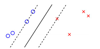
Figure 1.
Support vector classification for the separable case. The hyperplane is the solid line and the distance between the two dashed lines is the margin M. Points on the dashed line are the support vectors.


In this paper, we examine the usefulness of machine learning methods such as support vector machines, random forests and bagging for the extraction of information from the limit order book that can be used for intraday trading. For our empirical analysis, we first get 50 raw features from the LOBSTER message file and order book file of the iShares Core S & P 500 ETF for the time period from 27.06.2007 to 30.04.2019 and then construct 18 higher-level features (aggregated to 5 minutes frequency) which serve as predictors. Using straightforward specifications for the machine learning procedures and thereby avoiding excessive data snooping, we find that these procedures are unable to find high dimensional patterns in the order book that could be used for trading purposes. The observed significant predictability is mainly due to the inclusion of only one variable, namely the last price change, and is probably too small to ensure profitability once transaction costs are taken into account.
Citation: Manveer Kaur Mangat, Erhard Reschenhofer, Thomas Stark, Christian Zwatz. High-Frequency Trading with Machine Learning Algorithms and Limit Order Book Data[J]. Data Science in Finance and Economics, 2022, 2(4): 437-463. doi: 10.3934/DSFE.2022022
| [1] | Yongfeng Wang, Guofeng Yan . Survey on the application of deep learning in algorithmic trading. Data Science in Finance and Economics, 2021, 1(4): 345-361. doi: 10.3934/DSFE.2021019 |
| [2] | Mohamed F. Abd El-Aal . Analysis Factors Affecting Egyptian Inflation Based on Machine Learning Algorithms. Data Science in Finance and Economics, 2023, 3(3): 285-304. doi: 10.3934/DSFE.2023017 |
| [3] | Sami Mestiri . Credit scoring using machine learning and deep Learning-Based models. Data Science in Finance and Economics, 2024, 4(2): 236-248. doi: 10.3934/DSFE.2024009 |
| [4] | Wojciech Kuryłek . Can we profit from BigTechs' time series models in predicting earnings per share? Evidence from Poland. Data Science in Finance and Economics, 2024, 4(2): 218-235. doi: 10.3934/DSFE.2024008 |
| [5] | Angelica Mcwera, Jules Clement Mba . Predicting stock market direction in South African banking sector using ensemble machine learning techniques. Data Science in Finance and Economics, 2023, 3(4): 401-426. doi: 10.3934/DSFE.2023023 |
| [6] | Sangjae Lee, Joon Yeon Choeh . Exploring the influence of online word-of-mouth on hotel booking prices: insights from regression and ensemble-based machine learning methods. Data Science in Finance and Economics, 2024, 4(1): 65-82. doi: 10.3934/DSFE.2024003 |
| [7] | Mohamed F. Abd El-Aal . Determinants of Egypt's unemployment rate with machine learning algorithms. Data Science in Finance and Economics, 2024, 4(3): 333-349. doi: 10.3934/DSFE.2024014 |
| [8] | Jiawei He, Roman N. Makarov, Jake Tuero, Zilin Wang . Performance evaluation metric for statistical learning trading strategies. Data Science in Finance and Economics, 2024, 4(4): 570-600. doi: 10.3934/DSFE.2024024 |
| [9] | Paarth Thadani . Financial forecasting using stochastic models: reference from multi-commodity exchange of India. Data Science in Finance and Economics, 2021, 1(3): 196-214. doi: 10.3934/DSFE.2021011 |
| [10] | Lindani Dube, Tanja Verster . Enhancing classification performance in imbalanced datasets: A comparative analysis of machine learning models. Data Science in Finance and Economics, 2023, 3(4): 354-379. doi: 10.3934/DSFE.2023021 |
In this paper, we examine the usefulness of machine learning methods such as support vector machines, random forests and bagging for the extraction of information from the limit order book that can be used for intraday trading. For our empirical analysis, we first get 50 raw features from the LOBSTER message file and order book file of the iShares Core S & P 500 ETF for the time period from 27.06.2007 to 30.04.2019 and then construct 18 higher-level features (aggregated to 5 minutes frequency) which serve as predictors. Using straightforward specifications for the machine learning procedures and thereby avoiding excessive data snooping, we find that these procedures are unable to find high dimensional patterns in the order book that could be used for trading purposes. The observed significant predictability is mainly due to the inclusion of only one variable, namely the last price change, and is probably too small to ensure profitability once transaction costs are taken into account.
A proven method for the directional forecasting of financial time series would clearly be of great practical value. Unfortunately, empirical evidence of predictability is often impaired by the nonstationarity of these time series. Their statistical characteristics as well as their relationships with economic and political variables change over time. For example, the Monday-effect (see, e.g., Krämer 1998), the turn-of-the-month effect (see, e.g., Lakonishok and Smidt, 1988; Reschenhofer, 2010), and the positive first-order autocorrelation vanished over time (Reschenhofer et al., 2020b). In this regard, high-frequency data have a certain advantage over daily or monthly data because the prediction of the former is usually not based on stable patterns or relationships. Machine learning methods are used instead. Changes over time can easily be taken into account by rebuilding the model periodically, e.g., every year. The sorry practice of dividing the whole observation period in a learning period and a testing period and thereby building the model only once is completely incomprehensible. A dubious advantage of this practice is that it makes it easier to obscure data snooping. While an automatic and transparent approach is required if the model is rebuilt repeatedly, the one-time model building allows the unnoticed fiddling about with the model design and the tuning parameters. The fact that empirical studies of high-frequency data typically use extremely short observation periods is clearly not helpful in this regard. For example, Cont (2011) used thirty minutes, Zheng et al. (2012) and Kercheval and Zhang (2015) four hours and one day, respectively, Ntakaris et al. (2018) and Nousi et al. (2019) ten days, Gao et al. (2021) one month, and Kearns and Nevmyvaka (2013) two years. Kearns and Nevmyvaka (2013) examined the application of machine learning to the problem of predicting near-term price movements (as measured by the bid-ask midpoint) from limit order book data. They found profitable predictive signals but warned that the midpoint is a fictitious, idealized price and profitability is more elusive once trading costs (spread-crossing) are taken into account. Learning was performed for each of nineteen equities using all 2008 data and testing was performed using all 2009 data. Using prices and volumes at different levels of the limit order book and employing support vector machines, Kercheval and Zhang (2015) also found indications of short-term predictability of price movements. Their dataset covers a complete trading day for five stocks listed at the Nasdaq. The features extracted from this dataset included the prices and volumes for ten levels of the ask and bid side of the order book as well as bid-ask spreads. They used support vector machines with various feature sets and evaluated their models with cross validation. However, they did not test their forecasting procedure in a realistic trading experiment but used only a period of four hours to carry out some sort of plausibility check. Nousi et al. (2019) and Han et al. (2015) also found indications for the predictability of mid-price movements using similar sets of features but different observation periods (ten days and thirty minutes, respectively) and other machine learning algorithms (neural networks and random forests, respectively) in addition to support vector machines. Finally, indications of directional predictability were also found in the case of high-frequency exchange rates by Frömmel and Lampaert (2016) and, more directly, by Cai and Zhang (2016), who observed that trading strategies based on their directional forecasts were no longer profitable once transaction costs were accounted for. In this paper we propose a general methodological framework for the construction of machine learning based trading strategies for high frequency limit order data, which also includes a detailed account of the data cleaning procedure. We subsequently put it to effect using the support vector machine algorithm, which we apply to a fairly large limit order book dataset covering slightly more than eleven years. Thereby we consciously avoid tailoring the design of the forecasting procedures for the dataset at hand. Instead, we rather give an overview of the possible results that can be obtained with straightforward specifications. The support vector machine algorithm and the data set are described in Sections 2 and 3, respectively. Section 4 gives a thorough step by step description of the methodological framework. Section 5 presents the empirical results and briefly discusses the results obtained with other machine learning algorithms. Section 6 concludes.
Before providing a description of the binary support vector machine learning algorithm, we first recall basic terminology used in the machine learning context. The aim of binary classifiers is to categorize an observation xt=(xt1,…,xtp)∈Rp, p≥1, into one of two classes after being trained using a training set. The training set consists of observations that have already been classified.
Indeed, suppose we have a set of n observations x1,…,xn∈Rp falling into one of two classes yt∈{−1,1}, where t=1,…,n, then the training set T is defined by
| T={(xt,yt)|1≤t≤n}, | (1) |
where yt is the label of xt, Rp is the feature space, the components xti, i∈{1,…,p}, of xt∈Rp are the features and xt is the feature vector. Utilizing this training set T, we aim to construct prediction models, that will enable us to - as accurately as possible - predict the class of the next k observations contained in a specified evaluation set E
| E={(xt,yt)|n+1≤t≤n+k}. | (2) |
In order to obtain these prediction models, we use the support vector machine learning algorithm which we briefly describe in the following subsection.
When a linear separation between the class of observations xt with yt=−1 and the class of observations xt with yt=1 is possible, we want to compute the optimal separating (affine) hyperplane
| g(x)=xTβ+β0=0,β∈Rp,β0∈R | (3) |
that maximizes the margin M between both classes, see Figure 1.
In particular we want to find a hyperplane g(x)=xTβ+β0=0, such that
| g(x)=xTβ+β0≥1 for xi with yi=1, | (4) |
| g(x)=xTβ+β0≤−1 for xi with yi=−1. | (5) |
Then the corresponding decision function is given by
| f(x)=sign(xTβ+β0). | (6) |
In Figure 1, the blue points xb on the dashed line satisfy g(x)=xTβ+β0=−1 and the red points xr on the dashed line satisfy g(x)=xTβ+β0=1. So the margin, i.e. the distance between the two dashed lines, is given by
| M=|βxr+β0|‖β‖+|βxb+β0|‖β‖=2‖β‖, | (7) |
where ‖β‖=√∑pi=1β2i is the Euclidean norm. Hence finding the optimal, i.e. largest, margin is equivalent to solving the following optimization problem
| minβ,β012‖β‖2 | (8) |
| subject to yi(xTiβ+β0)≥1,i=1,…,n. | (9) |
Since we have a constrained minimization problem, we use the Lagrange multiplier method to solve it. In particular we minimize the Lagrangian (primal) function
| LP=12‖β‖2−n∑i=1αi(yi(xTiβ+β0)−1) | (10) |
with respect to β and β0. Setting the respective derivatives to zero results in the following criteria
| n∑i=1αiyi=0 and β=n∑i=1αiyixi. | (11) |
Substituting the criteria (11) into LP, we obtain the dual optimization problem
| maxn∑i=1αi−12n∑i=1n∑j=1αiαjyiyjxTixj | (12) |
| subject to n∑i=1αiyi=0,αi≥0,i=1,…,n. | (13) |
Using β=∑ni=1αyixi, the decision function is therefore given by
| f(x)=sign(n∑i=1αiyixTxi+β0). | (14) |
When the two classes are not linearly separable, training observations xi∈Rp will be missclassified, i.e sign(yi)≠sign(xTiβ+β0). Therefore in this case, we define slack variables ξ1,…,ξn∈R+ and allow some data points to be on the wrong side of the margin, i.e. ξi≤1, or on the wrong side of the hyperplane, i.e. ξi>1, by using the constraints
| g(x)=xTβ+β0≥1−ξi for xi with yi=1, | (15) |
| g(x)=xTβ+β0≤−1+ξi for xi with yi=−1, | (16) |
(see Figure 2).

Hence the optimal hyperplane can be obtained by solving the following optimization problem
| minβ,β012‖β‖2+Cn∑i=1ξi | (17) |
| subject to yi(xTiβ+β0)≥1−ξi, | (18) |
| ξi≥0,i=1,…,n, | (19) |
or equivalently by solving its corresponding dual problem obtained by applying the Lagrange multiplier method used above
| maxn∑i=1αi−12n∑i=1n∑j=1αiαjyiyjxTixj subject to n∑i=1αiyi=0,0≤αi≤C,i=1,…,n, | (20) |
where C>0 is a tuning parameter specifying the cost of missclassification on the learning set. If C is small, the SVM will have a high tolerance for missclassified observations, resulting in wider margins (high bias, low variance). However when C is large, the SVM is heavily penalized for misclassified observations, hence resulting in narrower margins to avoid as many missclassifications as possible (low bias, high variance). Therefore as C increases the risk of overfitting increases.
The decision function in this case is also given by
| f(x)=sign(n∑i=1αiyixTxi+β0). | (21) |
A more sophisticated approach to attaining a separation of the two classes is to map the feature space Rp into a higher-dimensional (or even infinite-dimensional) space, i.e. ϕ(x)∈Rq, x∈Rp, where p<<q and then to apply the aforementioned optimal margin hyperplane algorithm (20) in the higher dimension. The Lagrange dual function is then given by
| LD=n∑i=1αi−12n∑i=1n∑j=1αiαjyiyj⟨ϕ(xi),ϕ(xj)⟩, | (22) |
where ⟨ϕ(xi),ϕ(xj)⟩=ϕ(xi)Tϕ(xj) and the corresponding decision function by
| f(x)=sign(n∑i=1αiyi⟨ϕ(x),ϕ(xi)⟩+β0). | (23) |
Note that the optimization problem (22) and its solution (23) only contain the observations xi via dot products. In particular, it is not necessary to specify ϕ and therefore the dimension q as long as a suitable kernel function K
| K(xi,xj)=⟨ϕ(xi),ϕ(xj)⟩,i,j=1,…,n, | (24) |
is used. In particular, admissible kernel functions K(xi,xj) should be symmetric and positive (semi)definite.
Commonly used kernels are the linear kernel
| K(xj,xj′)=p∑i=1xjixj′i, | (25) |
the polynomial kernel
| K(xj,xj′)=p∑i=1(1+xjixj′i)d, | (26) |
where d>0 is the degree of the polynomial, and the radial kernel
| K(xj,xj′)=exp(−γp∑i=1(xji−xj′i)2), | (27) |
where γ>0. Just like for the cost parameter C, the SVM tries to increasingly avoid any missclassifications as the value of γ increases. Hence a too large value of γ runs the risk of overfitting the data.
In this section we describe the high frequency limit order book data sets used to construct features for the machine learning algorithms presented above. Using the online limit order book data tool LOBSTER, we download the data corresponding to the stock of interest after defining the relevant time period. Thereby LOBSTER provides two files: the message book and the order book file. The message book contains information about each trading event including its time of occurrence (in seconds after midnight with decimal precision of at least milliseconds), its type (submission of a new limit order, cancelation (partial deletion of a limit order), deletion (total deletion of a limit order), execution of a visible limit order, execution of a hidden limit order), its unique order ID, its size (number of shares), its price (dollar price times 10000) and finally whether a buy (1) or sell (-1) limit order is initiated (see Table 1). The corresponding order book is a list which contains unexecuted limit orders for both ask and bid for a specified level l. Thereby each level provides four values (ask price, ask volume, bid price, bid volume) with level 1 corresponding to the limit order with the best ask price, ask volume, bid price, bid volume and level 2 corresponding to the limit order with the second best ask price, ask volume, bid price, bid volume etc. (see Table 2). As to be expected, the evolution of the message book file results in a change in the order book file. Indeed, the k-th row in the message book facilitates the change in the order book from line k−1 to line k. For instance, as a result of the limit order deletion (event type 3) in the second line of the message book (Table 1), 100 shares from the ask side at price 118600 are omitted. This removal corresponds to the change in the order book (Table 2) from line 1 to 2. Accordingly, the best ask volume drops 9484 to 9384 shares.
| Time (sec) | Event Type | Order Id | Size | Price | Direction |
| ⋮ | ⋮ | ⋮ | ⋮ | ⋮ | ⋮ |
| 34713.685155243 | 1 | 206833312 | 100 | 118600 | -1 |
| 34714.133632201 | 3 | 206833312 | 100 | 118600 | 1 |
| ⋮ | ⋮ | ⋮ | ⋮ | ⋮ | ⋮ |
 DownLoad:
CSV
DownLoad:
CSV
| Ask Price 1 | Ask Size 1 | Bid Price 1 | Bid Size 1 | Ask Price 2 | Ask Size 2 | Bid Price 2 | Bid Size 2 | ⋮ |
| ⋮ | ⋮ | ⋮ | ⋮ | ⋮ | ⋮ | ⋮ | ⋮ | ⋮ |
| 1186600 | 9484 | 118500 | 8800 | 118700 | 22700 | 118400 | 14930 | ⋮ |
| 1186600 | 9384 | 118500 | 8800 | 118700 | 22700 | 118400 | 14930 | ⋮ |
| ⋮ | ⋮ | ⋮ | ⋮ | ⋮ | ⋮ | ⋮ | ⋮ | ⋮ |
DownLoad:
CSV
The flowchart in Figure 3 gives an overview of our proposed methodology. Utilizing high-frequency limit order book data, the aim is to construct new trading strategies based on the support vector machine algorithm. To evaluate the performance of a trading strategy, it is imperative to use a suitable benchmark for comparison. Indeed, in case the regarded stock exhibits a long-term upward trend, the benchmark strategy is always long (buy and hold strategy) and when the regarded stock exhibits a downward trend, the benchmark is constantly short in the stock. Thereby our objective is to predict one step ahead: using the information at time t, we want to forecast whether to buy (mid-quote return positive or constant) or sell (mid-quote return negative) our stock at time t+1.

The first step entails downloading the data from LOBSTER:
For each of the n trading days of the regarded stock, we download a message file and an orderbook file (up to level 5) from LOBSTER. For each 1-second interval, we extract 20 values from the orderbook file (the best ask price, the best ask volume, the best bid price, the best bid volume, …, the 5-th best ask price, the 5-th best ask volume, the 5-th best bid price, the 5-th best bid volume) and 30 values from the message file (see variables 21-50 in Table 3), resulting in 50 raw features (Table 3). To obtain the values for the 1-second intervals, we extract the value of the regarded features at the beginning of each second contained within the trading hours (9:00 am - 4:30 pm), which amounts to m = 6.5 hours × 60 minutes × 60 seconds = 23,400 seconds, hence 23,400 values for each feature per trading day.
| 1) Pask1,t | 2) Vask1,t | 3) Pbid1,t | 4) Vbid1,t | 5) Pask2,t |
| 6) Vask2,t | 7) Pbid2,t | 8) Vbid2,t | 9) Pask3,t | 10) Vask3,t |
| 11) Pbid3,t | 12) Vbid3,t | 13) Pask4,t | 14) Vask4,t | 15) Pbid4,t |
| 16) Vbid4,t | 17) Pask5,t | 18) Vask5,t | 19) Pbid5,t | 20) Vbid5,t |
| 21) BOn | 22) BOap | 23) BOmax | 24) SOn | 25) SOap |
| 26) SOmin | 27) pdBOn | 28) pdBOap | 29) pdBOmax | 30) pdSOn |
| 31) pdSOap | 32) pdSOmin | 33) tdBOn | 34) tdBOap | 35) tdBOmax |
| 36) tdSOn | 37) tdSOap | 38) tdSOmin | 39) evBOn | 40) evBOap |
| 41) evBOmax | 42) evSOn | 43) evSOap | 44) evSOmin | 45) ehBOn |
| 46) ehBOap | 47) ehBOmax | 48) ehSOn | 49) ehSOap | 50) ehSOmin |
DownLoad:
CSV
The next step entails cleaning the data:
Before the data can be used, it is subject to thorough processing. Clearly, every algorithm will perform poorly if it is fed with raw unfiltered data. It is crucial to analyze the data at hand before conducting any kind of data cleaning procedure, as applying a fixed set of filters could potentially lead to the loss of vital information.
With that in mind, we present two different data cleaning procedures, where the first cleansing process is specifically designed for the price and volume variables (variables 1-20 from Table 3), while the second cleaning procedure is defined for the remaining 30 variables from Table 3.
The data cleansing process for the level price and volume variables can be divided into four steps. First, the daily percentage of missing values for each of the variables are computed. If the magnitude of the missing values is extensive, the respective day is discarded.
The next step entails capturing extreme values of the price and volume variables and explicitly identifying these as non-available data points. Which measures can be used to detect extreme values? Given the nature of our regarded variables (volume and price levels), an obvious choice is the following collection of relative spreads:
| Pspr1,t=(Pask1,t−Pbid1,t)/Pask1,tPsprj,t=(Paskj,t−Pask1,t)/Paskj,t,2≤j≤5Psprj+4,t=(Pbid1,t−Pbidj,t)/Pbid1,t2≤j≤5. | (28) |
Indeed, using 0.015 as a benchmark, we identify the entry of a variable at time t as non-available, when the corresponding spread exhibits a value greater than 0.015, i.e.
| Pspr1,t>0.015⟹Paskj,t,Pbidj,t←NA, for j=1,…,5Psprj,t>0.015⟹Paskj,t…,Pask5,t,Vaskj,t,…,Vask5,t←NA, 2≤j≤5,Psprj,t>0.015⟹Pbidj−4,t…,Pbid5,t,Vbidj−4,t…,Vbid5,t←NA, 6≤j≤9, | (29) |
where NA indicates that the value at time t is classified as non-available.
Furthermore we only retain the values of Vaskj,t (Vbidj,t) whose corresponding level price Paskj,t (Pbidj,t) does not deviate more than 4 cents from the best ask price Pask1,t (bid price Pbid1,t), i.e.
| Paskj,t−Pask1,t>0.04⟹Vaskj,t←NA, for j=1,…,5Pbid1,t−Pbidj,t>0.04⟹Vbidj,t←NA, for j=1,…,5 | (30) |
In the last step, we additionally compute the log returns of Pask1,t, Pbid1,t and the mid-quote prices (Pbid1,t+Pask1,t)/2 to identify whole days opposed to single values of the variables at a time t, that need to be removed due to extreme values. Indeed, as soon as a return greater than 0.015 is detected, the whole respective day is completely removed.
This concludes the data cleaning process for the level ask and volume prices. The cleansing procedure for the last 30 variables from Table 3 consists of only two steps. Once again we compute the daily percentage of missing values for each of the variables and discard the respective day in case of a large number of missing values. In contrast to the data cleaning procedure applied to the volume and price variables, we conduct a visual inspection of the last 30 variables from Table 3, by plotting the variables against time to identify any potential outliers. Once these are identified, their corresponding values are set to missing concluding the cleansing procedure.
Having cleaned the data set, the next step is to select and define relevant features:
In addition to the cleaned features from the previous section, we define additional features, using the cleaned price and level features, that can be categorized into three groups: 1) spreads 2) volumes and 3) returns (see Table 4).
| Feature Category | Feature |
| Spreads | X1,t=(Pask1,t−Pbid1,t)/Pask1,t |
| Xj,t=(Paskj,t−Pask1,t)/Paskj,t,2≤j≤5 | |
| Xj+4,t=(Pbid1,t−Pbidj,t)/Pbid1,t2≤j≤5 | |
| Volumes | X10,t=log(Vask1,t) |
| X11,t=log(Vbid1,t) | |
| X12,t=log(5∑j=1Vaskj,t1{Paskj,t−Pask1,t<0.04}) | |
| X13,t=log(5∑j=1Vbidj,t1{Pbid1,t−Pbidj,t<0.04}) | |
| X14,t=X12,t+X13,t | |
| X15,t=X12,t/X13,t | |
| Returns | X16,t=log(Pask1,t)−log(Pask1,t−1) |
| X17,t=log(Pbid1,t)−log(Pbid1,t−1) | |
| X18,t=log((Pask1,t+Pbid1,t)/2)−log((Pask1,t−1+Pbid1,t−1)/2) |
DownLoad:
CSV
For uniformity reasons, we henceforth denote the cleaned features from Table 3 by Xbasici,t i=1,…,50 (e.g. X1,t corresponds to the variable 1 in Table 3, X2,t to the variable 2 etc.) and define X as the set of all features, i.e.
| X={Xbasic1,t,…,Xbasic50,t,X1,t,…,X18,t} | (31) |
containing all the p=68 considered features.
Due to the sampling frequency of one second, the features in Table 3 and 4 are inevitably polluted by microstructure noise which is caused by the bid-ask spread, the discreteness of price changes, asynchronous trading, etc.. A common way to reduce the impact of this problem is to perform data aggregation. In particular, we conduct a 5-minute data aggregation procedure reducing the number of data points from 23400 to 78 per day for each variable, adjusting the time stamps accordingly (see Figure 4).

Clearly in order to aggregate the variables, one has to carefully choose a measure, that gives an accurate representation of the variable values within the considered aggregation interval. To aggregate the return variables (X16,t,X17,t,X18,t), we simply compute the telescoping sums: we add 300 one second returns to obtain 5 min returns
| Xj,˜t=300˜t∑t=1+(˜t−1)300Xj,t+1−Xj,t,˜t=1,2,3,…,(nm/300), | (32) |
for j∈{16,17,18}, where n is the total number of regarded trading days and m=23400 (amount of seconds contained in each trading day).
For the basic features (Xbasic1,t−Xbasic50,t), spread features (X1,t−X9,t) and volume features (X10,t-X15,t), we apply a trimmed mean (discard 10% on either ends) to each of the 78 300-second intervals contained in a trading day, to obtain the aggregated variables. We illustrate its application with an example: consider the following sequence of values (Xhj,t)300t=1, which consists of the first 300 entries of the feature Xhj,t, corresponding to the first 5 minute interval on the first trading day, where (j,h)∈I={(j,basic)|j=1,…,50}∪{(j,.)|j=1,…,18}. The first step consists of computing the order statistics, i.e. arranging the values in ascending order Xhj,(1)≤Xhj,(2),…,≤Xhj,(300). Subsequently, 10% of the observations are removed from either sides, which amounts to 30 values being removed. Hence more generally we have
| Xhj,˜t=1300−2l300˜t−l∑t=1+(˜t−1)300+lXhj,(t)˜t=1,2,3…,(nm/300), | (33) |
for (j,h)∈I, where l=300∗α with α=0.10. Henceforth we denote X as the set of all p=68 aggregated features:
| X={Xbasic1,…,Xbasic50,X1,…,X18}, | (34) |
where Xhj=(Xhj,1,…,Xhj,(nm/300))∈X with (j,h)∈I. Note, as we are interested in the one step ahead forcast (i.e we want to predict the trading signal for time t+1 using the information at time t), our regarded features are lagged by nature. Evidently, the number p of features can be increased significantly by additionally including lagged features. In particular, we additionally consider features that are doubly lagged, hence increasing the number of features from p to 2p. We denote the corresponding set as LX. For illustration: the lagged features on the first day would be given by (Xhj,2,Xhj,3,…,Xhj,77) and the corresponding doubly lagged features as (Xhj,1,Xhj,2,…,Xhj,76), (j,h)∈I. Lastly, due to their varying scales (e.g. volume vs. spread), we standardize all features. Once the features are established, we can proceed to construct training and evaluation sets:
In order to define training and evaluation sets, the feature vectors have to be provided with appropriate labels. Using the feature vector at time ˜t, we want to predict the directional movement of the mid-quote stock returns at time ˜t+1, to determine whether to buy or sell our stock at time ˜t+1. Hence with the dependant variable given by
| Y˜t={1if X18,˜t≥0−1if X18,˜t<0, | (35) |
we define the training set as L={(x˜t,y˜t)}, where either x˜t∈Rp with p∈{1,…,68} or x˜t∈R2p with 2p∈{2,4,…,2∗68} (depending on the inclusion of doubly lagged features) is the feature vector at time ˜t and y˜t∈{−1,1} is the corresponding true label indicating whether a buy signal (Y~t+1=1) or sell signal (Y~t+1=−1) is generated at time ˜t+1.
When regarding the feature set X, which by definition consists of lagged variables, the features at time ˜t are used to forecast the value of the dependent variable at time ˜t+1. Hence to construct the training and evaluation sets, the 78-th (last) entry has to be omitted from each day of the feature vectors, while the first entry has to be omitted from the dependant variable Y every day to obtain the appropriate corresponding labels (see Figure 5.a).

However, when regarding the feature set LX, which consists of lagged Xhj and additionally doubly lagged features LXhj, the number of possible labels and predictions diminish from 77 to 76 per day (see Figure 5.b).
Having established the appropriate labels for the features, we next have to determine the size of the training and evaluation sets. In contrast to the studies by Kercheval and Zhang (2015), Nousi et al. (2019) and Kearns and Nevmyvaka (2013), we use much larger limit order book data sets that cover slightly more than eleven years. We use a whole trading year, consisting of 250 days, to form our training set to see whether we can capture annual trends and characteristics of the regarded data. Since depending on the inclusion of additionally lagged features, each day provides us with u∈{76,77} pairs of data points, our training set T consists of 250u pairs.
The training set T is succeeded by the evaluation set E, which also covers a whole trading year and is used to determine how well the machine learning model has learned from the training set T. As the statistical characteristics of financial time series change over time, we continuously update our training and evaluation set, in order to keep up with changing trends and patterns in the limit-order book data. We employ a 250-days shifting window approach (see Figure 6): using the first 250 days (250u data points) (training set T1), the intraday buy and sell signals of the subsequent 250 days (250u values) (evaluation set E1) are predicted, then E1 is used as the training set T2 to once again predict the intraday buy and sell signals for the subsequent 250 days (evaluation set E2) etc. until the last training and evaluation set.

Once the training and evaluation sets are established, the next step entails defining meaningful tuning parameters of the regarded machine learning algorithm.
Depending on the algorithm to be implemented, one has to first specify single or multiple tuning parameters. How should the tuning parameters be chosen? Clearly, before the tuning procedure can be conducted, a feature set ˉx∈Rp has to be selected first, where depending on the inclusion of doubly lagged features p∈{1,…,68} or p∈{2,4,…,2∗68}. While the task of selecting features is based on the trial and error approach and hence varies significantly across different cases, a general guideline for selecting features for tuning procedures is to use a modest amount of features that cover the whole spectrum of available information as well as possible. Once the feature set ˉx is established, there are two ways to find possibly useful tuning parameters.
The common way is to regard various models that adopt a wide spectrum of tuning parameter values or tuning parameter combinations, when more than one tuning parameter is involved, and to compute their predictive performance (Accuracy) to establish which tuning parameter or tuning parameter combination yields the best result, i.e. exhibit the highest number of correct classifications. When using the 250-day shifting window approach, this translates into computing
| PP=(n250−1)(1250u(l−1)250u+250u∑k=(l−1)250u+11yk=˜yk),l=1,…,(n/250)−1,u∈{76,77}, |
where yk is the actual label (trading signal) and ˜yk is the predicted label. Recall, u=77 when the lagged features are used and u=76, when the double lagged features are additionally included.
The second way to find possibly useful tuning parameters entails plots of cumulative returns. For various values of a tuning parameter or for various combinations of tuning parameters (in case of more than one tuning parameter), we can depict the cumulative returns of the corresponding trading strategies generated by the machine learning methods. This is a highly effective method to analyze how the performance of competing trading strategies change over time and to identify which strategies deliver good results in different time periods. Using solely the total sum of returns as a measure for the trading performance can be severely misleading hence it is imperative to consider the evolution of the cumulative sums over time. Indeed, suppose we have a trading strategy that outperforms the benchmark in the distant past (e.g. 2010-2015) but then underperforms it in the recent past (e.g. 2016-2017). Then the total sum corresponding to this strategy might still be a lot higher than that of the benchmark although its performance was inferior in the recent past - which is clearly of relevance - therefore delivering a deceptive result.
Thereby, for fixed values of a tuning parameter or parameters, the first training set T1, corresponding to the first 250 days, is used to train the model, after which the model provides a trading signal, i.e. y˜t for each of the feature vectors x˜t contained in the evaluation set E1. Due to the 250 days shifting window approach, this process is repeated with E1 being used as the training set T2 to train the model, so that the model can predict the trading signals for the feature vectors x˜t in E2. This is repeated until the last training and evaluation sets are reached. Then the cumulative returns are obtained by multiplying the predicted trading signals y˜t, with the corresponding returns X18,˜t, i.e.
| Sτ=τ∑˜t=250∗u+1X18,˜t+1y˜t,τ=250u+2,250u+3,…,nu and u=77 | (36) |
| Sτ=τ∑˜t=250∗u+1X18,˜t+2y˜t,τ=250u+2,250u+3,…,nu and u=76 | (37) |
with S250u+1=X18,250u+2∗y250u+1 for u=77 and S250u+1=X18,250∗u+3∗y250u+1 for u=76, depending on the inclusion of additionally lagged features (see Figure 5).
This approach has the following advantage over the tuning procedure based on predictive performance: The predictive performance only differentiates between correct and incorrect classifications and does not allow for different degrees of misclassifications. For instance, when a buy signal for a significantly small (absolute) negative return is generated, it clearly has a smaller overall effect on the cumulative return than when a buy signal is generated for a larger (absolute) negative return. While this concept can be clearly illustrated by plots of cumulative returns, the predictive performance evaluation method is too limited to capture this concept. Indeed, it does not matter how small or large the (absolute) negative return is, a misclassification in that case is just that: a missclassification.
Once the "optimal" tuning parameters are found, the next step entails finding the "optimal" feature vector. Clearly, considering the set of all features, there is a generous amount of feature vectors that can be constructed. Trying every single combination will inevitably pose significant challenges with regard to computer memory (size) and computing power (speed), hence it is crucial to choose feature vectors systematically. We therefore propose the following procedure, where we only consider the features X1−X18: First we start off by considering 1-dimensional feature vectors Xi, i=1,…,18, to establish the feature Xi∈X, which provides the most profitable 1-dimensional trading strategy. Secondly, including Xi, we regard all 2-dimensional feature vectors x=(Xi,Xj), where j∈{1,…,18}∖{i}, to once again determine which 2-dimensional feature vector corresponds to the most profitable strategy. This process can be repeatedly applied. Thereby the resulting k-dimensional feature vector ˉx∈Rk, where 1≤k<<18 consists of k−1 fixed features and a varying k−th feature, which covers all the features with the exception of the k−1 features that are already included as a fixed component. Note, as the mid-quote returns X18 are based on best ask and best bid prices, the information content of X18 does not significantly vary from that provided by the ask X16 and bid X17 returns. Hence if one of the features Xj, j∈{16,17,18} is contained in the feature vector ˉx and Xi with i∈{16,17,18}∖{j}, then it suffices to either only include Xi or Xj.
In the last step, we repeat the above mentioned process by additionally including the lagged variables of each respective feature, therefore doubling the number of predictors contained in each feature vector and reducing the number of predictions to 76 from 77 per day.
Subsequently we can establish which feature vector ˆx delivers the optimal output. Hence the optimal prediction model is given by the machine learning algorithm equipped with 1) the tuning parameters obtained by following the procedure in Section 4.6 and 2) the feature vector ˆx obtained by following the process described above.
We now proceed to apply our methodology to high-frequency data:
For our empirical analysis we download the message and order book file data of the iShares Core S & P 500 ETF (IVV) from LOBSTER and extract the features presented in Table 3 as described in Section 4.1 for the time period 27.06.2007 to 30.04.2019, resulting in n=2980 trading days.
Subsequently we proceed with cleaning the data: We first conduct the data cleaning procedure for the price and volume variables (variables 1-20 from Table 3). As a result of the first step, which entails computing the daily percentage of missing values, we remove 27 early-closure days (the day before Independence Day, the day after Thanksgiving, and Christmas Eve, respectively) and, in addition, January 9, 2019 due to their large amount of daily missing values. Secondly, when the relative spreads (28) are greater than 0.015, we set the values of the thereby affected variables to missing as described in (29). Third, we examine the log volumes for outliers. As Figure A1 clearly illustrates, our data does not exhibit any outliers, hence there is no need to set additional values to missing. After that we set level volumes at time t∈{1,2,3,…,(m2980)} to missing, whose corresponding level prices at time t significantly deviate from the best price (first level price) at time t (see (30)). In the last step, we compute the log mid-quote, ask and bid returns to identify and consequently omit days that exhibit a return greater than 0.015, which leads to the elimination of the following days: September 19, 2008, May 6, 2010 and August 24. Hence in total 2949 days remain. We then conduct the data cleaning procedure of the remaining 30 variables (variables 31-50 from Table 3). As for the price and volume variables, we first compute the daily percentage of missing values for each of these variables. Thereby the last 30 variables exhibit a considerable amount of missing values per day (see Figure A2 - note, since variable j, for j∈{21,24,27,30,33,36,39,42,45,48}, is used to construct variable j+1 and j+2, it is sufficient to compute the missing values for variable j only). Omitting these days, leads to a significantly minor set of remaining days for each of the last 30 variables. Hence due to their sparse information content we discard these variables. Lastly we compute the features presented in Table 4 before applying the data aggregation procedure from Section 4.4, to obtain Xj,˜t j=1,…,18 and Xbasici,˜t i=1,…,20. However, since Xj,˜t j=1,…,18 are defined using Xbasici,˜t i=1,…,50, we henceforth only regard the features Xj,˜t j=1,…,18 to avoid repetition of information content, hence p=18.
Subsequently, we utilize the 250 day shifting window approach to train and evaluate our machine learning models. Note, since our data set covers 2949 days in total, our last evaluation set only consists of 199 opposed to 250 days (see Figure 7).

As described in Section 4.6, a feature set to be used in the course of the tuning procedure of the respective machine learning algorithm has to be defined. As we regard three categories of features: 1) spreads (X1,˜t−X9,˜t), 2) volumes (X10,˜t−X15,˜t) and 3) returns variables (X16,˜t−X18,˜t), we use a representative of each class to cover the range of these categories. In particular, we regard the following feature vector
| ˉx=(X1,X15,X18), | (38) |
to conduct the tuning procedure.
Once the optimal tuning parameters are established, the next step entails finding the optimal feature vector such that the trading strategy generated by the corresponding machine learning model is the overall most profitable. Following Section 4.7, we first start off by considering 1-dimensional feature vectors Xj, where j∈ J={1,…,18}, to establish which feature Xj∈X facilitates the generation of the most profitable trading strategy. Depending on the most informative feature Xj j∈J, we systematically define a collection of feature vectors (see Table A1 in the appendix) and subsequently use these for the optimization procedure to establish which feature vector translates into the most profitable strategy.
Having established the features, training and evaluation sets, as well as the feature vector to be used for the tuning procedure in addition to the collection of feature vectors that are to be used for the optimization process, we can finally proceed with applying the machine learning algorithm from Section 2. Thereby, due to the overall increasing trend of the regarded ETF, the buy and hold strategy (always long) is used as a benchmark when using the approach of plots of cumulative returns to compare the performance of competing trading strategies. For all our computations, we use the free statistical software R R2021 and in particular the R package e1071 to implement the machine learning algorithms:
As seen in Section 2.1, the support vector machine algorithm has different numbers of tuning parameters depending on the choice of the kernel. Indeed, in case of a linear kernel there is one parameter (cost C) to be tuned, in case of a polynomial kernel there are two (cost C and degree d of the polynomial) and lastly for the radial kernel there are also two parameters (cost C and γ, accounting for the smoothness of the decision boundary) to be tuned. Thereby there is no general consensus on what kernel and subsequently what tuning values to choose. For instance, Kercheval and Zhang (2015) employ the SVM algorithm using the polynomial kernel of order two and set the cost parameter C to 0.25 when working with LOB data, claiming that different choices for C do not have a significant affect on the results. On the other hand Nousi at al. (2019), also using LOB data, used a linear kernel and specified the cost parameter C by performing a 3-fold cross-validation on the training set, where possible values for C ranged from 0.00001 to 0.1.
For our empirical analysis we use the radial kernel, which requires the specification of two tuning parameters: γ and C. In Section 4.6, two different methods to determine the optimal tuning parameters were presented. Here we consider the method based on the plots of cumulative returns (see Table A2 and Table A3 in the appendix for the predictive performance of different models). Using the feature vector (38), we regard a generous amount of values for the tuning parameters to establish which combination of tuning values results in the most profitable trading strategy (see Figure 8). In particular we optimize over the following set A,
| A={(γ,C)|γ∈Γ,C∈ˉC}, | (39) |

where Γ={0.1,0.5,1,2,3,5,8,10} and ˉC={0.1,0.5,0.7,1,2,3,5,8,10,30,50,100}. The reason we consider values with minor differences (such as γ=0.1 and γ=0.5 or γ=2 and γ=3 or C=0.7 and C=1), is to determine whether this disparity is sufficient to facilitate the production of vastly different results or whether there is barely any difference to be noticed. Note, to capture the range of the values, we regard values at the lower, middle and high end of the spectrum for both γ and the cost parameter C.
A visual inception of Figure 8, where each subplot corresponds to a fixed value of γ with varying values of γ, shows that overall there are four optimal tuning pairs that approximately achieve the same result: A1={(0.1,C)|C∈{10,30}} and A2={(1,C)|C∈{5,10}}. Note that the trading strategies corresponding to the tuning pairs contained in A1 (A2) either coincide or exhibit an insignificant difference as can be seen in Figure 8.a (Figure 8.b). This supports the idea, that the choice of the cost parameters C do not significantly influence the outcome of a strategy, as long as they do not differ vastly. Having four tuning pairs to select from, we choose (γ,C)=(0.1,10) to conduct our further analysis. The choice of C=10 is straightforward, as (0.1,10)∈A1 and (1,10)∈A2, the selection of γ=0.1 over γ=1 is discretionary.
Having defined the optimal tuning parameters, we now proceed to systematically define a collection of feature vectors as proposed in Table A1, to establish which of these feature vectors deliver the most profitable trading strategy. Thereby the first step entails regarding all 1-dimensional feature vectors x=Xj∈X, j=1,…,18, to determine which feature is the most informative, i.e. results in the most superior trading strategy (see Figure 9.a). As Figure 9.a clearly illustrates, the return variables are the most informative with the bid returns Xi=16 (red) taking a slight lead, the lagged (II−IV) and doubly lagged (II∗−IV∗) feature vectors from Table 5 are of relevance (obtained from Table A1 in the Appendix). Finally, using feature vectors from Table 5, we can define the SVM models with the tuning parameters (γ,C)=(0.1,10) and the 250-day shifting window approach to determine which feature vector ˆx translates into the most profitable trading strategy (see Figure 9.c-h.).

| Lags | Feature Vectors |
| 1 | II: (X18,˜t,Xj,˜t)j∈J∖{18} |
| III: (X18,˜t,X1,˜t,Xj,˜t)j∈J∖{1,18} | |
| IV: (X18,˜t,X1,˜t,X15,˜t,Xj,˜t)j∈J∖{1,15,18} | |
| 2 | II∗: (X18,˜t,X18,˜t−1,Xj,˜t−1,Xj,˜t)j∈J∖{18} |
| III∗: (X18,˜t,X18,˜t−1,X1,˜t,X1,˜t−1,Xj,˜t−1,Xj,˜t)j∈J∖{1,18} | |
| IV∗: (X18,˜t,X18,˜t−1,X1,˜t,X1,˜t−1,X15,˜t,X15,˜t−1,Xj,˜t−1,Xj,˜t)j∈J∖{1,15,18} |
DownLoad:
CSV
A visual inspection of Figure 9 shows, that the feature vector corresponding to the optimal strategy, is given by ˆx=(X18,˜t,X1,˜t,X15,˜t). Generally the feature vectors containing return variables (corresponding to red, darkred and gold in Figure 9) exhibit the best performance. Thereby the inclusion of additional features does not necessarily result in a better outcome (for instance, compare Figure 9.c to Figure 9.d or Figure 9.g to Figure. 9 h). Furthermore note that including the second lags does not enhance the performance of the models. In fact, as Figure 9h clearly illustrates, the performance of the trading strategies significantly decline (lower total cumulative sum) in comparison to their single lagged counterpart in Figure 9.d.
Hence according to our empirical analysis, the SVM model using the tuning parameters (γ,C)=(0.1,10) and the feature vector ˆx=(X18,˜t,X1,˜t,X15,˜t) generates the optimal trading strategy.
In a previous study on volatility forecasting (see Reschenhofer et al. 2020a), we also used the iShares Core S & P 500 ETF. However, since large outliers occur more frequently in stock returns than in index returns, we examined additionally also a collection of fifteen DJIA-components. The results obtained with the index ETF were corroborated by the results obtained with the individual stocks. We assume that the same is true for the present study, particularly because outliers are less of a concern in directional forecasting than in volatility forecasting.
In this subsection, the results obtained with support vector machines are compared with the results obtained with other machine learning algorithms. Figures 10, 11 and 12 display the results obtained by using the random forest algorithm with 3000 trees, bagging with an interaction depth of 4 and 3000 trees, and the k-nearest neighbors algorithm with 300 neighbors, respectively, using the exact same feature sets that were used to analyze the performance of the trading strategies based on the SVM algorithm in Figure 9. Obviously, there are no major differences in the performance between the different machine learning algorithms. Again, feature vectors containing return variables generally exhibit the best performance and the inclusion of additional features does not necessarily result in a better outcome. Also the inclusion of the second lags does not enhance the performance.


In their review of recent studies on financial forecasting and trading, Reschenhofer et al. (2020b) identified many weaknesses such as unsuitable benchmarks, too short evaluation periods and nonoperational trading strategies. Their main conclusion was that apparently good forecasting performance does, in general, not translate into profitability once realistic transaction costs and the effect of data snooping are taken into account. While in the case of high-frequency trading, some peculiarities of intraday returns, e.g., autocorrelation, can straightforwardly be employed for directional forecasting (see Reschenhofer et al. 2020a, for the application to volatility forecasting and Hansen and Lunde, 2006, for general issues related to market microstructure noise), the adequate consideration of transaction costs requires the precise knowledge of the order book at any time and is therefore extremely difficult if not impossible (because of the critical dependence on the amount to be invested). However, it is quite clear that the costs of frequent trading are very high and can only be recouped if the prediction accuracy is very high. So the first step is to look for promising trading strategies in the absence of transaction costs. Employing machine learning models and rebuilding these models periodically, we hope to be able to find patterns which are stable over short to medium periods of time and can therefore be used to make profitable trading decisions. Indeed, we achieve significant predictability when we apply support vector machines to high-frequency order book data. However, the performance is only good but not great. It is comparable to the performance that could be achieved with simple methods in past periods of high autocorrelation in daily returns. There appears to be no extra gain due to high frequency, high dimensionality and artificial intelligence (machine learning). Again, we must assume that most of the possible profits will be eaten up by the transaction costs (most notably the bid-ask spread). The steady decrease in transaction costs over time is offset by the increase in trading frequency when we switch from daily trading to intraday trading. The observed predictability is mainly due to the inclusion of only one variable, namely the last price change, whereby it is irrelevant whether we use bid prices, ask prices or mid prices. The inclusion of additional variables from the order book does not result in any significant improvement (see Figure 9). We obtain similar findings when we use random forests (see Figure 10) or bagging (see Figure 11) or a k-nearest neighbors algorithm (see Figure 12) instead of support vector machines. In this paper we proposed trading strategies based on machine learning algorithms with specifically very straightforward specifications as the aim was to provide a overall general framework for the construction of trading strategies by consciously avoiding excessive data snooping. As we were unable to find high dimensional patterns in the order book that could be used for trading purposes, our findings imply that the construction of better performing trading strategies might inevitably rely on being tailored to the regarded dataset at hand (data snooping).
The authors are grateful to Nikolaus Hautsch for facilitating the access to LOBSTER. This research did not receive any specific grant from funding agencies in the public, commercial, or not-for-profit sectors.
All authors declare no conflicts of interest in this paper.
| [1] |
Cai C, Zhang Q (2016) High-frequency exchange rate forecasting. Eur Financ Manage 22: 120–141. https://doi.org/10.1111/eufm.12052 doi: 10.1111/eufm.12052

|
| [2] |
Cont R (2011) Statistical modeling of high-frequency financial data. IEEE Signal Proces Mag 28: 16–25. https://doi.org/10.1109/MSP.2011.941548 doi: 10.1109/MSP.2011.941548
|
| [3] |
Fletcher T, Shawe-Taylor J (2013) Multiple kernel learning with fisher kernels for high frequency currency prediction. Computat Econ 42: 217–240. https://doi.org/10.1007/s10614-012-9317-z doi: 10.1007/s10614-012-9317-z
|
| [4] |
Frömmel M, Lampaert K (2016) Does frequency matter for intraday technical trading? Financ Res Lett 18: 177–183. https://doi.org/10.1016/j.frl.2016.04.014 doi: 10.1016/j.frl.2016.04.014
|
| [5] |
Gao K, Luk W, Weston S (2021) High-Frequency Trading and Financial Time-Series Prediction with Spiking Neural Networks. Wilmott 18–33. https://doi.org/10.1002/wilm.10927 doi: 10.1002/wilm.10927
|
| [6] | Han J, Hong J, Sutardja N, et al. (2015) Machine learning techniques for price change forecast using the limit order book data. Working Paper. |
| [7] |
Hansen P, Lunde A (2006) Realized variance and market microstructure noise. J Bus Econ Stat 24: 127–161. https://doi.org/10.1198/073500106000000071 doi: 10.1198/073500106000000071
|
| [8] |
Huang W, Nakamori Y, Wang S (2005) Forecasting stock market movement direction with support vector machine. Comput opera res 32: 2513–2522. https://doi.org/10.1016/j.cor.2004.03.016 doi: 10.1016/j.cor.2004.03.016
|
| [9] | Kearns M, Nevmyvaka Y (2013) Machine learning for market microstructure and high frequency trading. High Frequency Trading: New Realities for Traders, Markets, and Regulators Risk Books London, UK |
| [10] |
Kercheval A, Zhang Y (2015) Modelling high-frequency limit order book dynamics with support vector machine. Quantitat Financ 15: 1315–1329. https://doi.org/10.1080/14697688.2015.1032546 doi: 10.1080/14697688.2015.1032546
|
| [11] |
Krämer W (1998) Note Short-term predictability of German stock returns. Empir Econ 23: 635–639. https://doi.org/10.1007/s001810050040 doi: 10.1007/s001810050040
|
| [12] | Krollner B, Vanstone Bruce, Finnie G (2010) inancial time series forecasting with machine learning techniques: a survey. ESANN, |
| [13] |
Lakonishok J and Smidt S (1988) Are seasonal anomalies real? A ninety-year perspective. Rev financ stud 1: 403–425. https://doi.org/10.1093/rfs/1.4.403 doi: 10.1093/rfs/1.4.403
|
| [14] | LOBSTER: Limit Order Book System - The Efficient Reconstructer. LOBSTER Team. Available from: https://lobsterdata.com/info/DataStructure.php. |
| [15] |
Majhi R, Panda G, Sahoo G (2009) Development and performance evaluation of FLANN based model for forecasting of stock markets. Expert syst Appl 36: 6800–6808. https://doi.org/10.1016/j.eswa.2008.08.008 doi: 10.1016/j.eswa.2008.08.008
|
| [16] |
Nousi P, Tsantekidis A, Passalis N, et al. (2019) Machine learning for forecasting mid-price movements using limit order book data. Ieee Access 7: 64722–64736. https://doi.org/10.1109/ACCESS.2019.2916793 doi: 10.1109/ACCESS.2019.2916793
|
| [17] |
Ntakaris A, Magris M, Kanniainen J, et al. (2018) Benchmark dataset for mid-price forecasting of limit order book data with machine learning methods. J Forecast 37: 852–866. https://doi.org/10.1002/for.2543 doi: 10.1002/for.2543
|
| [18] | R: A Language and Environment for Statistical Computing, R Foundation for Statistical Computing. Available from: http://www.R-project.org/. |
| [19] | Reschenhofer E (2010) Further evidence on the turn-of-the-month effect. Bus Econ J. |
| [20] |
Reschenhofer E, Mangat M, Stark T (2020a), Volatility forecasts, proxies and loss functions J Empir Financ 59: 133–153. https://doi.org/10.1016/j.jempfin.2020.09.006 doi: 10.1016/j.jempfin.2020.09.006
|
| [21] |
Reschenhofer E, Mangat M, Zwatz C et al. (2020b), Evaluation of current research on stock return predictability. J Forecast 39: 334–351. https://doi.org/10.1002/for.2629 doi: 10.1002/for.2629
|
| [22] |
Tay F, Cao L (2019) Application of support vector machines in financial time series forecasting. omega 29: 309–317. https://doi.org/10.1016/S0305-0483(01)00026-3 doi: 10.1016/S0305-0483(01)00026-3
|
| [23] | Tran D, Kanniainen J, Gabbouj M et al. (2019) Data-driven neural architecture learning for financial time-series forecasting. arXiv preprint arXiv: 1903.06751 https://doi.org/10.48550/arXiv.1903.06751 |
| [24] | Zheng B, Moulines E andAbergel F (2012) Price jump prediction in limit order book arXiv preprint arXiv: 1204.1381 https://doi.org/10.48550/arXiv.1204.1381 |
 DSFE-02-04-022-s001.pdf DSFE-02-04-022-s001.pdf |
 |
| 1. | Mohammad El Hajj, Jamil Hammoud, Unveiling the Influence of Artificial Intelligence and Machine Learning on Financial Markets: A Comprehensive Analysis of AI Applications in Trading, Risk Management, and Financial Operations, 2023, 16, 1911-8074, 434, 10.3390/jrfm16100434 | |
| 2. | Visalakshi Palaniappan, Iskandar Ishak, Hamidah Ibrahim, Fatimah Sidi, Zuriati Ahmad Zukarnain, A Review on High-Frequency Trading Forecasting Methods: Opportunity and Challenges for Quantum Based Method, 2024, 12, 2169-3536, 167471, 10.1109/ACCESS.2024.3418458 | |
| 3. | Partap Singh, 2024, chapter 7, 9798369378274, 145, 10.4018/979-8-3693-7827-4.ch007 | |
| 4. | Zhenghui Li, Yanting Xu, Ziqing Du, Valuing financial data: The case of analyst forecasts, 2025, 75, 15446123, 106847, 10.1016/j.frl.2025.106847 | |
| 5. | Elias Dritsas, Maria Trigka, Exploring the Intersection of Machine Learning and Big Data: A Survey, 2025, 7, 2504-4990, 13, 10.3390/make7010013 |
Manveer Kaur Mangat, Erhard Reschenhofer, Thomas Stark, Christian Zwatz. High-Frequency Trading with Machine Learning Algorithms and Limit Order Book Data[J]. Data Science in Finance and Economics, 2022, 2(4): 437-463. doi: 10.3934/DSFE.2022022

| Time (sec) | Event Type | Order Id | Size | Price | Direction |
| ⋮ | ⋮ | ⋮ | ⋮ | ⋮ | ⋮ |
| 34713.685155243 | 1 | 206833312 | 100 | 118600 | -1 |
| 34714.133632201 | 3 | 206833312 | 100 | 118600 | 1 |
| ⋮ | ⋮ | ⋮ | ⋮ | ⋮ | ⋮ |
DownLoad:
CSV
| Ask Price 1 | Ask Size 1 | Bid Price 1 | Bid Size 1 | Ask Price 2 | Ask Size 2 | Bid Price 2 | Bid Size 2 | ⋮ |
| ⋮ | ⋮ | ⋮ | ⋮ | ⋮ | ⋮ | ⋮ | ⋮ | ⋮ |
| 1186600 | 9484 | 118500 | 8800 | 118700 | 22700 | 118400 | 14930 | ⋮ |
| 1186600 | 9384 | 118500 | 8800 | 118700 | 22700 | 118400 | 14930 | ⋮ |
| ⋮ | ⋮ | ⋮ | ⋮ | ⋮ | ⋮ | ⋮ | ⋮ | ⋮ |
DownLoad:
CSV
| 1) Pask1,t | 2) Vask1,t | 3) Pbid1,t | 4) Vbid1,t | 5) Pask2,t |
| 6) Vask2,t | 7) Pbid2,t | 8) Vbid2,t | 9) Pask3,t | 10) Vask3,t |
| 11) Pbid3,t | 12) Vbid3,t | 13) Pask4,t | 14) Vask4,t | 15) Pbid4,t |
| 16) Vbid4,t | 17) Pask5,t | 18) Vask5,t | 19) Pbid5,t | 20) Vbid5,t |
| 21) BOn | 22) BOap | 23) BOmax | 24) SOn | 25) SOap |
| 26) SOmin | 27) pdBOn | 28) pdBOap | 29) pdBOmax | 30) pdSOn |
| 31) pdSOap | 32) pdSOmin | 33) tdBOn | 34) tdBOap | 35) tdBOmax |
| 36) tdSOn | 37) tdSOap | 38) tdSOmin | 39) evBOn | 40) evBOap |
| 41) evBOmax | 42) evSOn | 43) evSOap | 44) evSOmin | 45) ehBOn |
| 46) ehBOap | 47) ehBOmax | 48) ehSOn | 49) ehSOap | 50) ehSOmin |
DownLoad:
CSV
| Feature Category | Feature |
| Spreads | X1,t=(Pask1,t−Pbid1,t)/Pask1,t |
| Xj,t=(Paskj,t−Pask1,t)/Paskj,t,2≤j≤5 | |
| Xj+4,t=(Pbid1,t−Pbidj,t)/Pbid1,t2≤j≤5 | |
| Volumes | X10,t=log(Vask1,t) |
| X11,t=log(Vbid1,t) | |
| X12,t=log(5∑j=1Vaskj,t1{Paskj,t−Pask1,t<0.04}) | |
| X13,t=log(5∑j=1Vbidj,t1{Pbid1,t−Pbidj,t<0.04}) | |
| X14,t=X12,t+X13,t | |
| X15,t=X12,t/X13,t | |
| Returns | X16,t=log(Pask1,t)−log(Pask1,t−1) |
| X17,t=log(Pbid1,t)−log(Pbid1,t−1) | |
| X18,t=log((Pask1,t+Pbid1,t)/2)−log((Pask1,t−1+Pbid1,t−1)/2) |
DownLoad:
CSV
| Lags | Feature Vectors |
| 1 | II: (X18,˜t,Xj,˜t)j∈J∖{18} |
| III: (X18,˜t,X1,˜t,Xj,˜t)j∈J∖{1,18} | |
| IV: (X18,˜t,X1,˜t,X15,˜t,Xj,˜t)j∈J∖{1,15,18} | |
| 2 | II∗: (X18,˜t,X18,˜t−1,Xj,˜t−1,Xj,˜t)j∈J∖{18} |
| III∗: (X18,˜t,X18,˜t−1,X1,˜t,X1,˜t−1,Xj,˜t−1,Xj,˜t)j∈J∖{1,18} | |
| IV∗: (X18,˜t,X18,˜t−1,X1,˜t,X1,˜t−1,X15,˜t,X15,˜t−1,Xj,˜t−1,Xj,˜t)j∈J∖{1,15,18} |
DownLoad:
CSV
| Time (sec) | Event Type | Order Id | Size | Price | Direction |
| ⋮ | ⋮ | ⋮ | ⋮ | ⋮ | ⋮ |
| 34713.685155243 | 1 | 206833312 | 100 | 118600 | -1 |
| 34714.133632201 | 3 | 206833312 | 100 | 118600 | 1 |
| ⋮ | ⋮ | ⋮ | ⋮ | ⋮ | ⋮ |
| Ask Price 1 | Ask Size 1 | Bid Price 1 | Bid Size 1 | Ask Price 2 | Ask Size 2 | Bid Price 2 | Bid Size 2 | ⋮ |
| ⋮ | ⋮ | ⋮ | ⋮ | ⋮ | ⋮ | ⋮ | ⋮ | ⋮ |
| 1186600 | 9484 | 118500 | 8800 | 118700 | 22700 | 118400 | 14930 | ⋮ |
| 1186600 | 9384 | 118500 | 8800 | 118700 | 22700 | 118400 | 14930 | ⋮ |
| ⋮ | ⋮ | ⋮ | ⋮ | ⋮ | ⋮ | ⋮ | ⋮ | ⋮ |
| 1) Pask1,t | 2) Vask1,t | 3) Pbid1,t | 4) Vbid1,t | 5) Pask2,t |
| 6) Vask2,t | 7) Pbid2,t | 8) Vbid2,t | 9) Pask3,t | 10) Vask3,t |
| 11) Pbid3,t | 12) Vbid3,t | 13) Pask4,t | 14) Vask4,t | 15) Pbid4,t |
| 16) Vbid4,t | 17) Pask5,t | 18) Vask5,t | 19) Pbid5,t | 20) Vbid5,t |
| 21) BOn | 22) BOap | 23) BOmax | 24) SOn | 25) SOap |
| 26) SOmin | 27) pdBOn | 28) pdBOap | 29) pdBOmax | 30) pdSOn |
| 31) pdSOap | 32) pdSOmin | 33) tdBOn | 34) tdBOap | 35) tdBOmax |
| 36) tdSOn | 37) tdSOap | 38) tdSOmin | 39) evBOn | 40) evBOap |
| 41) evBOmax | 42) evSOn | 43) evSOap | 44) evSOmin | 45) ehBOn |
| 46) ehBOap | 47) ehBOmax | 48) ehSOn | 49) ehSOap | 50) ehSOmin |
| Feature Category | Feature |
| Spreads | X1,t=(Pask1,t−Pbid1,t)/Pask1,t |
| Xj,t=(Paskj,t−Pask1,t)/Paskj,t,2≤j≤5 | |
| Xj+4,t=(Pbid1,t−Pbidj,t)/Pbid1,t2≤j≤5 | |
| Volumes | X10,t=log(Vask1,t) |
| X11,t=log(Vbid1,t) | |
| X12,t=log(5∑j=1Vaskj,t1{Paskj,t−Pask1,t<0.04}) | |
| X13,t=log(5∑j=1Vbidj,t1{Pbid1,t−Pbidj,t<0.04}) | |
| X14,t=X12,t+X13,t | |
| X15,t=X12,t/X13,t | |
| Returns | X16,t=log(Pask1,t)−log(Pask1,t−1) |
| X17,t=log(Pbid1,t)−log(Pbid1,t−1) | |
| X18,t=log((Pask1,t+Pbid1,t)/2)−log((Pask1,t−1+Pbid1,t−1)/2) |
| Lags | Feature Vectors |
| 1 | II: (X18,˜t,Xj,˜t)j∈J∖{18} |
| III: (X18,˜t,X1,˜t,Xj,˜t)j∈J∖{1,18} | |
| IV: (X18,˜t,X1,˜t,X15,˜t,Xj,˜t)j∈J∖{1,15,18} | |
| 2 | II∗: (X18,˜t,X18,˜t−1,Xj,˜t−1,Xj,˜t)j∈J∖{18} |
| III∗: (X18,˜t,X18,˜t−1,X1,˜t,X1,˜t−1,Xj,˜t−1,Xj,˜t)j∈J∖{1,18} | |
| IV∗: (X18,˜t,X18,˜t−1,X1,˜t,X1,˜t−1,X15,˜t,X15,˜t−1,Xj,˜t−1,Xj,˜t)j∈J∖{1,15,18} |
