The mast cell/S1P axis is not linked to pre-lesional male skin remodeling in a mouse model of eczema

Ross M. Tanis; Piper A. Wedman-Robida; Alena P. Chumanevich; John W. Fuseler; Carole A. Oskeritzian; Ross M. Tanis; Piper A. Wedman-Robida; Alena P. Chumanevich; John W. Fuseler; Carole A. Oskeritzian

doi:10.3934/Allergy.2021012

AIMS Allergy and Immunology

2021, Volume 5, Issue 3: 160-174. doi: 10.3934/Allergy.2021012

Previous Article Next Article

Research article

The mast cell/S1P axis is not linked to pre-lesional male skin remodeling in a mouse model of eczema

1.
Department of Pathology, Microbiology and Immunology, University of South Carolina School of Medicine, Columbia, SC 29209, USA
2.
Department of Internal Medicine, Loyola University Medical Center, 2160 South 1st Avenue, Maywood, IL 60153, USA
3.
Department of Natural Science, Northwestern Oklahoma State University, Science Building 100-D, 709 Oklahoma Boulevard, Alva, OK 73717, USA
† These two authors contributed equally.

Received: 25 March 2021 Accepted: 25 May 2021 Published: 28 May 2021

Atopic dermatitis (AD, eczema) is an inflammatory skin condition whose histopathology involves remodeling. Few preclinical AD studies are performed using male mice. The histopathological mechanisms underlying AD development were investigated here in male mice at a pre-lesional stage using a human AD-like mouse model. Hypodermal cellular infiltration without thickening of skin layers was observed after one epicutaneous exposure to antigen ovalbumin (OVA), compared to controls. In contrast to our previous report using female mice, OVA treatment did not activate skin mast cells (MC) or elevate sphingosine-1-phosphate (S1P) levels while increasing systemic but not local levels of CCL2, CCL3 and CCL5 chemokines. In contrast to the pathogenic AD mechanisms we recently uncovered in female, S1P-mediated skin MC activation with subsequent local chemokine production is not observed in male mice, supporting sex differences in pre-lesional stages of AD. We are proposing that differential involvement of the MC/S1P axis in early pathogenic skin changes contributes to the well documented yet still incompletely understood sex-dimorphic susceptibility to AD in humans.
- pathogenesis,
- mast cells,
- sphingosine-1-phosphate,
- chemokines,
- animal models,
- eczema
Citation: Ross M. Tanis, Piper A. Wedman-Robida, Alena P. Chumanevich, John W. Fuseler, Carole A. Oskeritzian. The mast cell/S1P axis is not linked to pre-lesional male skin remodeling in a mouse model of eczema[J]. AIMS Allergy and Immunology, 2021, 5(3): 160-174. doi: 10.3934/Allergy.2021012

Related Papers:

Abstract

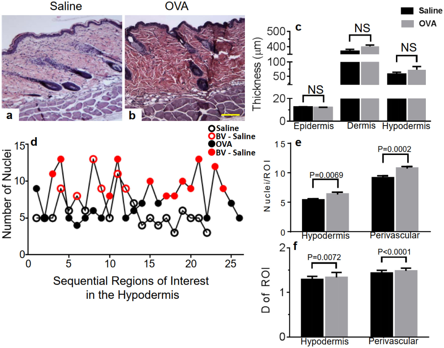
Atopic dermatitis (AD, eczema) is an inflammatory skin condition whose histopathology involves remodeling. Few preclinical AD studies are performed using male mice. The histopathological mechanisms underlying AD development were investigated here in male mice at a pre-lesional stage using a human AD-like mouse model. Hypodermal cellular infiltration without thickening of skin layers was observed after one epicutaneous exposure to antigen ovalbumin (OVA), compared to controls. In contrast to our previous report using female mice, OVA treatment did not activate skin mast cells (MC) or elevate sphingosine-1-phosphate (S1P) levels while increasing systemic but not local levels of CCL2, CCL3 and CCL5 chemokines. In contrast to the pathogenic AD mechanisms we recently uncovered in female, S1P-mediated skin MC activation with subsequent local chemokine production is not observed in male mice, supporting sex differences in pre-lesional stages of AD. We are proposing that differential involvement of the MC/S1P axis in early pathogenic skin changes contributes to the well documented yet still incompletely understood sex-dimorphic susceptibility to AD in humans.

Abbreviations

atopic dermatitis

OVA

ovalbumin

MCs

mast cells

S1P

sphingosine-1-phosphate

blood vessels

Acknowledgments

We thank VCU Lipidomics/Metabolomics Core for lipid determinations, which is supported by the National Institutes of Health (NIH)/NCI Cancer Center Support grant P30 CA016059 to the VCU Massey Cancer Center and by a shared resource grant S10RR031535. We thank Ahmed Aladami for technical assistance. This work was supported by the National Institute of Allergy and Infectious Diseases/NIH R01 AI095494, the National Institute of Arthritis and Musculoskeletal and Skin Diseases/NIH R21 AR067996 and a National Institute of General Medical Sciences/NIH Bioinformatics Pilot Project P20 GM103499 to CAO.

Conflict of interest

All authors declare no conflicts of interest in this paper.

Author contributions

Conception and study design: PAWR and CAO; Development of methodology: PAWR, APC, RMT, JWF and CAO; Acquisition of data: RMT, PAWR, APC, JWF; Analysis and interpretation of data: RWT, PAWR, APC, JWF, CAO; Technical support: APC, JWF; Writing, review and/or revision of the manuscript: RWT, PAWR, APC, JWF, CAO.

References

[1]	Hanifin JM, Reed ML (2007) A population-based survey of eczema prevalence in the United States. Dermatitis 18: 82-91.
[2]	Silverberg JI (2017) Public health burden and epidemiology of atopic dermatitis. Dermatol Clin 35: 283-289.
[3]	Thyssen JP, Johansen JD, Linneberg A, et al. (2010) The epidemiology of hand eczema in the general population—prevalence and main findings. Contact Dermatitis 62: 75-87.
[4]	Harrop J, Chinn S, Verlato G, et al. (2007) Eczema, atopy and allergen exposure in adults: a population-based study. Clin Exp Allergy 37: 526-535.
[5]	Chen W, Mempel M, Schober W, et al. (2008) Gender difference, sex hormones, and immediate type hypersensitivity reactions. Allergy 63: 418-1427.
[6]	Lee JH, Haselkorn T, Chipps BE, et al. (2006) Gender differences in IgE-mediated allergic asthma in the epidemiology and natural history of asthma: outcomes and treatment regimens (TENOR) study. J Asthma 43: 179-184.
[7]	Simpson CR, Newton J, Hippisley-Cox J, et al. (2009) Trends in the epidemiology and prescribing of medication for eczema in England. J Roy Soc Med 102: 108-117.
[8]	Osman M, Hansell AL, Simpson CR, et al. (2007) Gender-specific presentations for asthma, allergic rhinitis and eczema in primary care. Prim Care Respir J 16: 28-35.
[9]	Silverberg JI, Hanifin JM (2013) Adult eczema prevalence and associations with asthma and other health and demographic factors: a US population-based study. J Allergy Clin Immun 132: 1132-1138.
[10]	Ridolo E, Incorvaia C, Martignago I, et al. (2019) Sex in respiratory and skin allergies. Clin Rev Allerg Immu 56: 322-332.
[11]	Fuxench ZCC, Block JK, Boguniewicz M, et al. (2019) Atopic dermatitis in America study: a cross-sectional study examining the prevalence and disease burden of atopic dermatitis in the US adult population. J Invest Dermatol 139: 583-590.
[12]	Sacotte R, Silverberg JI (2018) Epidemiology of adult atopic dermatitis. Clin Dermatol 36: 595-605.
[13]	Gutermuth J, Ollert M, Ring J, et al. (2004) Mouse models of atopic eczema critically evaluated. Int Arch Allergy Imm 135: 262-276.
[14]	Ewald DA, Noda S, Oliva M, et al. (2017) Major differences between human atopic dermatitis and murine models, as determined by using global transcriptomic profiling. J Allergy Clin Immun 139: 562-571.
[15]	Yoshihisa Y, Andoh T, Matsunaga K, et al. (2016) Efficacy of astaxanthin for the treatment of atopic dermatitis in a murine model. PLoS One 11: e0152288.
[16]	Brunner PM, Guttman-Yassky E, et al. (2017) The immunology of atopic dermatitis and its reversibility with broad-spectrum and targeted therapies. J Allergy Clin Immun 139: S65-S76.
[17]	Mu Z, Zhao Y, Liu X, et al. (2014) Molecular biology of atopic dermatitis. Clin Rev Allerg Immu 47: 193-218.
[18]	Wedman PA, Aladhami A, Chumanevich AP, et al. (2018) Mast cells and sphingosine-1-phosphate underlie prelesional remodeling in a mouse model of eczema. Allergy 73: 405-415.
[19]	Akdis CA, Bousquet J, Grattan CE, et al. (2019) Highlights and recent developments in skin allergy and related diseases in EAACI journals (2018). Clin Transl Allergy 9: 60.
[20]	Spergel JM, Mizoguchi E, Brewer JP, et al. (1998) Epicutaneous sensitization with protein antigen induces localized allergic dermatitis and hyperresponsiveness to methacholine after single exposure to aerosolized antigen in mice. J Clin Invest 101: 1614-1622.
[21]	Wolters PJ, Mallen-St Clair J, Lewis CC, et al. (2005) Tissue-selective mast cell reconstitution and differential lung gene expression in mast cell-deficient Kit(W-sh)/Kit(W-sh) sash mice. Clin Exp Allergy 35: 82-88.
[22]	Wedman P, Aladhami A, Beste M, et al. (2015) A new image analysis method based on morphometric and fractal parameters for rapid evaluation of in situ mammalian mast cell status. Microsc Microanal 21: 1573-1581.
[23]	Oskeritzian CA, Hait NC, Wedman P, et al. (2015) The sphingosine-1-phosphate/sphingosine-1-phosphate receptor 2 axis regulates early airway T-cell infiltration in murine mast cell-dependent acute allergic responses. J Allergy Clin Immun 135: 1008.
[24]	Odhiambo JA, Williams HC, Clayton TO, et al. (2009) Global variations in prevalence of eczema symptoms in children from ISAAC Phase Three. J Allergy Clin Immun 124: 1251-1258.
[25]	Pesce G, Marcon A, Carosso A, et al. (2015) Adult eczema in Italy: prevalence and associations with environmental factors. J Eur Acad Dermatol 29: 1180-1187.
[26]	Sandstrom MH, Faergemann J (2004) Prognosis and prognostic factors in adult patients with atopic dermatitis: a long-term follow-up questionnaire study. Brit J Dermatol 150: 103-110.
[27]	Wang G, Savinko T, Wolff H, et al. (2007) Repeated epicutaneous exposures to ovalbumin progressively induce atopic dermatitis-like skin lesions in mice. Clin Exp Allergy 37: 151-161.
[28]	Suárez-Fariñas M, Tintle SJ, Shemer A, et al. (2011) Nonlesional atopic dermatitis skin is characterized by broad terminal differentiation defects and variable immune abnormalities. J Allergy Clin Immun 127: 954-964.
[29]	Gaga M, Ong YE, Benyahia F, et al. (2008) Skin reactivity and local cell recruitment in human atopic and nonatopic subjects by CCL2/MCP-1 and CCL3/MIP-1alpha. Allergy 63: 703-711.
[30]	Mukai K, Tsai T, Saito H, et al. (2018) Mast cells as sources of cytokines, chemokines, and growth factors. Immunol Rev 282: 121-150.
[31]	Homey B, Steinhoff M, Ruzicka T, et al. (2006) Cytokines and chemokines orchestrate atopic skin inflammation. J Allergy Clin Immun 118: 178-189.
[32]	Su C, Yang T, Wu Z, et al. (2017) Differentiation of T-helper cells in distinct phases of atopic dermatitis involves Th1/Th2 and Th17/Treg. Eur J Inflammation 15: 46-52.
[33]	Ungar B, Garcet S, Gonzalez J, et al. (2017) An integrated model of atopic dermatitis biomarkers highlights the systemic nature of the disease. J Invest Dermatol 137: 603-613.
[34]	Brunner PM, Suárez-Fariñas M, He H, et al. (2017) The atopic dermatitis blood signature is characterized by increases in inflammatory and cardiovascular risk proteins. Sci Rep 7: 8707.
[35]	Lauffer F, Baghin V, Standl M, et al. (2021) Predicting persistence of atopic dermatitis in children using clinical attributes and serum proteins. Allergy 76: 1158-1172.
[36]	Sulcova J, Meyer M, Guiducci E, et al. (2015) Mast cells are dispensable in a genetic mouse model of chronic dermatitis. Am J Pathol 185: 1575-1587.
[37]	Sehra S, Serezani APM, Ocaña JA, et al. (2016) Mast cells regulate epidermal barrier function and the development of allergic skin inflammation. J Invest Dermatol 136: 1429-1437.
[38]	Groneberg DA, Bester C, Grützkau A, et al. (2005) Mast cells and vasculature in atopic dermatitis-potential stimulus of neoangiogenesis. Allergy 60: 90-97.
[39]	Oskeritzian CA, Milstien S, Spiegel S (2007) Sphingosine-1-phosphate in allergic responses, asthma and anaphylaxis. Pharmacol Therapeut 115: 390-399.
[40]	Price MM, Oskeritzian CA, Milstien S, et al. (2008) Sphingosine-1-phosphate synthesis and functions in mast cells. Future Lipidol 3: 665-674.
[41]	Oskeritzian CA, Alvarez SE, Hait NC, et al. (2008) Distinct roles of sphingosine kinases 1 and 2 in human mast cell functions. Blood 111: 4193-4200.
[42]	Oskeritzian CA, Price MM, Hait NC, et al. (2010) Essential roles of sphingosine-1-phosphate receptor 2 in human mast cell activation, anaphylaxis, and pulmonary edema. J Exp Med 207: 465-474.
[43]	Oskeritzian CA (2015) Mast cell plasticity and sphingosine-1-phosphate in immunity, inflammation and cancer. Mol Immunol 63: 104-112.
[44]	Chumanevich A, Wedman P, Oskeritzian CA (2016) Sphingosine-1-phosphate/sphingosine-1-phosphate receptor 2 axis can promote mouse and human primary mast cell angiogenic potential through upregulation of vascular endothelial growth factor-A and matrix metalloproteinase-2. Mediat Inflamm 2016: 1503206.
[45]	Holt PG, Britten D, Sedgwick JD (1987) Suppression of IgE responses by antigen inhalation: studies on the role of genetic and environmental factors. Immunology 60: 97-102.
[46]	Zaitsu M, Narita SI, Lambert KC, et al. (2007) Estradiol activates mast cells via a non-genomic estrogen receptor-alpha and calcium influx. Mol Immunol 44: 1977-1985.
[47]	Vliagoftis H, Dimitriadou V, Boucher W, et al. (1992) Estradiol augments while tamoxifen inhibits rat mast cell secretion. Int Arch Allergy Imm 98: 398-409.
[48]	Hox V, Desai A, Bandara G, et al. (2015) Estrogen increases the severity of anaphylaxis in female mice through enhanced endothelial nitric oxide synthase expression and nitric oxide production. J Allergy Clin Immun 135: 729-736.
[49]	Paller AS, Kabashima K, Bieber T (2017) Therapeutic pipeline for atopic dermatitis: end of the drought?. J Allergy Clin Immun 140: 633-643.
[50]	Chan S, Cornelius V, Cro S, et al. (2019) Treatment effects of omalizumab on severe pediatric atopic dermatitis: the ADAPT randomized clinical trail. JAMA Pediatr 174: 29-37.
[51]	Cruz-Orengo L, Daniels BP, Dorsey D, et al. (2014) Enhanced sphingosine-1-phosphate receptor 2 expression underlies female CNS autoimmunity susceptibility. J Clin Invest 124: 2571-2584.

Reader Comments

Your name:*

Email:*
© 2021 the Author(s), licensee AIMS Press. This is an open access article distributed under the terms of the Creative Commons Attribution License (http://creativecommons.org/licenses/by/4.0)