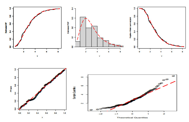
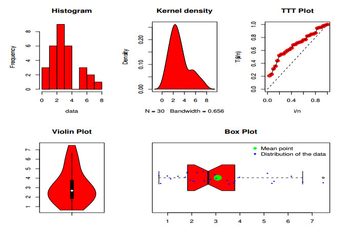
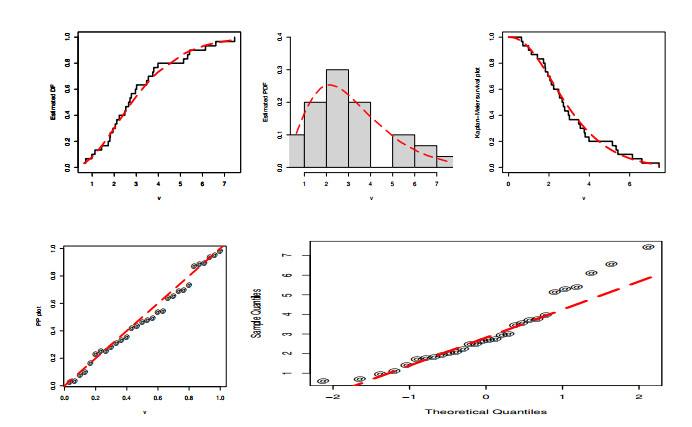
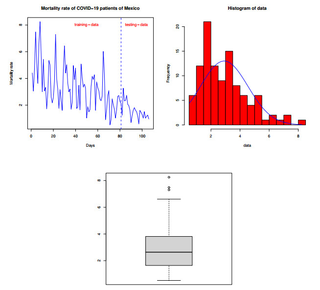
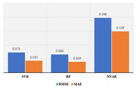
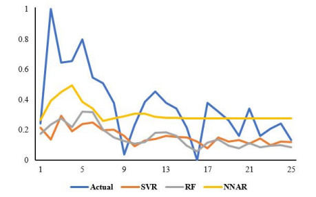
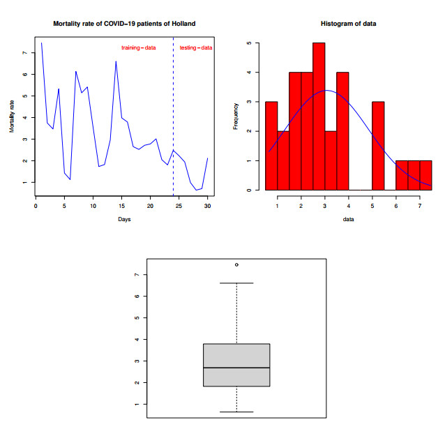
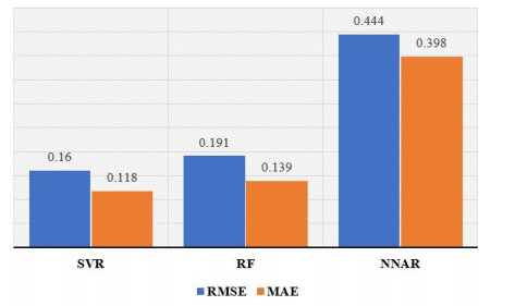
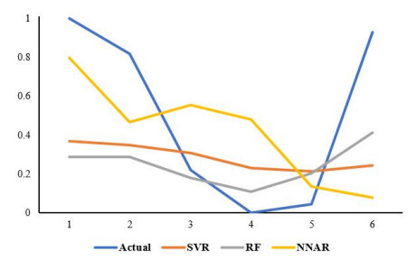
Statistical methodologies have broader applications in almost every sector of life including education, hydrology, reliability, management, and healthcare sciences. Among these sectors, statistical modeling and predicting data in the healthcare sector is very crucial. In this paper, we introduce a new method, namely, a new extended exponential family to update the distributional flexibility of the existing models. Based on this approach, a new version of the Weibull model, namely, a new extended exponential Weibull model is introduced. The applicability of the new extended exponential Weibull model is shown by considering two data sets taken from the health sciences. The first data set represents the mortality rate of the patients infected by the coronavirus disease 2019 (COVID-19) in Mexico. Whereas, the second set represents the mortality rate of COVID-19 patients in Holland. Utilizing the same data sets, we carry out forecasting using three machine learning (ML) methods including support vector regression (SVR), random forest (RF), and neural network autoregression (NNAR). To assess their forecasting performances, two statistical accuracy measures, namely, root mean square error (RMSE) and mean absolute error (MAE) are considered. Based on our findings, it is observed that the RF algorithm is very effective in predicting the death rate of the COVID-19 data in Mexico. Whereas, for the second data, the SVR performs better as compared to the other methods.
Citation: Yinghui Zhou, Zubair Ahmad, Zahra Almaspoor, Faridoon Khan, Elsayed tag-Eldin, Zahoor Iqbal, Mahmoud El-Morshedy. On the implementation of a new version of the Weibull distribution and machine learning approach to model the COVID-19 data[J]. Mathematical Biosciences and Engineering, 2023, 20(1): 337-364. doi: 10.3934/mbe.2023016
Statistical methodologies have broader applications in almost every sector of life including education, hydrology, reliability, management, and healthcare sciences. Among these sectors, statistical modeling and predicting data in the healthcare sector is very crucial. In this paper, we introduce a new method, namely, a new extended exponential family to update the distributional flexibility of the existing models. Based on this approach, a new version of the Weibull model, namely, a new extended exponential Weibull model is introduced. The applicability of the new extended exponential Weibull model is shown by considering two data sets taken from the health sciences. The first data set represents the mortality rate of the patients infected by the coronavirus disease 2019 (COVID-19) in Mexico. Whereas, the second set represents the mortality rate of COVID-19 patients in Holland. Utilizing the same data sets, we carry out forecasting using three machine learning (ML) methods including support vector regression (SVR), random forest (RF), and neural network autoregression (NNAR). To assess their forecasting performances, two statistical accuracy measures, namely, root mean square error (RMSE) and mean absolute error (MAE) are considered. Based on our findings, it is observed that the RF algorithm is very effective in predicting the death rate of the COVID-19 data in Mexico. Whereas, for the second data, the SVR performs better as compared to the other methods.

| [1] |
B. T. Ngo, P. Marik, P. Kory, L. Shapiro, R. Thomadsen, J. Iglesias, et al., The time to offer treatments for COVID-19, Expert Opin. Invest. Drugs, 30 (2021), 505–518. https://doi.org/10.1080/13543784.2021.1901883 doi: 10.1080/13543784.2021.1901883

|
| [2] |
B. Pfefferbaum, C. S. North, Mental health and the COVID-19 pandemic, N. Engl. J. Med., 383 (2020), 510–512. https://doi.org/10.1056/NEJMp2008017 doi: 10.1056/NEJMp2008017
|
| [3] |
E. J. Kim, L. Marrast, J. Conigliaro, COVID-19: magnifying the effect of health disparities, J. Gen. Intern. Med., 35 (2020), 2441–2442. https://doi.org/10.1007/s11606-020-05881-4 doi: 10.1007/s11606-020-05881-4
|
| [4] |
J. Campion, A. Javed, N. Sartorius, M. Marmot, Addressing the public mental health challenge of COVID-19, Lancet Psychiatry, 7 (2020), 657–659. https://doi.org/10.1016/S2215-0366(20)30240-6 doi: 10.1016/S2215-0366(20)30240-6
|
| [5] |
A. T. Gloster, D. Lamnisos, J. Lubenko, G. Presti, V. Squatrito, M. Constantinou, et al., Impact of COVID-19 pandemic on mental health: an international study, PloS One, 15 (2020), e0244809. https://doi.org/10.1371/journal.pone.0244809 doi: 10.1371/journal.pone.0244809
|
| [6] |
D. Talevi, V. Socci, M. Carai, G. Carnaghi, S. Faleri, E. Trebbi, et al., Mental health outcomes of the COVID-19 pandemic, Riv. Psichiatr., 55 (2020), 137–144. https://doi.org/10.1708/3382.33569 doi: 10.1708/3382.33569
|
| [7] |
E. A. Wastnedge, R. M. Reynolds, S. R. Van Boeckel, S. J. Stock, F. C. Denison, J. A. Maybin, et al., Pregnancy and COVID-19, Physiol. Rev., 101 (2021), 303–318. https://doi.org/10.1152/physrev.00024.2020 doi: 10.1152/physrev.00024.2020
|
| [8] |
W. Bo, Z. Ahmad, A. R. Alanzi, A. I. Al-Omari, E. H. Hafez, S. F. Abdelwahab, The current COVID-19 pandemic in China: an overview and corona data analysis, Alexandria Eng. J., 61 (2021), 1369–1381. https://doi.org/10.1016/j.aej.2021.06.025 doi: 10.1016/j.aej.2021.06.025
|
| [9] |
V. H. Moreau, Forecast predictions for the COVID-19 pandemic in Brazil by statistical modeling using the Weibull distribution for daily new cases and deaths, Braz. J. Microbiol., 51 (2020), 1109–1115. https://doi.org/10.1007/s42770-020-00331-z doi: 10.1007/s42770-020-00331-z
|
| [10] |
S. Tuli, S. Tuli, R. Tuli, S. S. Gill, Predicting the growth and trend of COVID-19 pandemic using machine learning and cloud computing, Internet Things, 11 (2020), 100222. https://doi.org/10.1016/j.iot.2020.100222 doi: 10.1016/j.iot.2020.100222
|
| [11] |
S. M. Rahman, J. Kim, B. Laratte, Disruption in Circularity? Impact analysis of COVID-19 on ship recycling using Weibull tonnage estimation and scenario analysis method, Resour. Conserv. Recycl., 164 (2021), 105139. https://doi.org/10.1016/j.resconrec.2020.105139 doi: 10.1016/j.resconrec.2020.105139
|
| [12] |
E. M. Almetwally, R. Alharbi, D. Alnagar, E. H. Hafez, A new inverted topp-leone distribution: applications to the COVID-19 mortality rate in two different countries, Axioms, 10 (2021), 25. https://doi.org/10.3390/axioms10010025 doi: 10.3390/axioms10010025
|
| [13] |
M. Alizadeh, G. M. Cordeiro, A. D. Nascimento, M. D. C. S. Lima, E. M. Ortega, Odd-Burr generalized family of distributions with some applications, J. Stat. Comput. Simul., 87 (2017), 367–389. https://doi.org/10.1080/00949655.2016.1209200 doi: 10.1080/00949655.2016.1209200
|
| [14] |
F. Chipepa, B. Oluyede, B. Makubate, A new generalized family of odd Lindley-G distributions with application, Int. J. Stat. Probab., 8 (2019), 1–22. https://doi.org/10.5539/ijsp.v8n6p1 doi: 10.5539/ijsp.v8n6p1
|
| [15] |
L. Handique, S. Chakraborty, T. A. de Andrade, The exponentiated generalized Marshall–Olkin family of distribution: its properties and applications, Ann. Data Sci., 6 (2019), 391–411. https://doi.org/10.1007/s40745-018-0166-z doi: 10.1007/s40745-018-0166-z
|
| [16] |
M. H. Tahir, M. A. Hussain, G. M. Cordeiro, M. El-Morshedy, M. S. Eliwa, A new Kumaraswamy generalized family of distributions with properties, applications, and bivariate extension, Mathematics, 8 (2020), 1989. https://doi.org/10.3390/math8111989 doi: 10.3390/math8111989
|
| [17] |
S. M. Zaidi, M. M. A. Sobhi, M. El-Morshedy, A. Z. Afify, A new generalized family of distributions: properties and applications, AIMS Math., 6 (2021), 456–476. https://doi.org/10.3934/math.2021028 doi: 10.3934/math.2021028
|
| [18] |
F. H. Riad, E. Hussam, A. M. Gemeay, R. A. Aldallal, A. Z. Afify, Classical and Bayesian inference of the weighted-exponential distribution with an application to insurance data, Math. Biosci. Eng., 19 (2022), 6551–6581. https://doi.org/10.3934/mbe.2022309 doi: 10.3934/mbe.2022309
|
| [19] |
M. E. Bakr, A. A. Al-Babtain, Z. Mahmood, R. A. Aldallal, S. K. Khosa, M. M. Abd El-Raouf, et al., Statistical modelling for a new family of generalized distributions with real data applications, Math. Biosci. Eng., 19 (2022), 8705–8740. https://doi.org/10.3934/mbe.2022404 doi: 10.3934/mbe.2022404
|
| [20] |
A. Xu, S. Zhou, Y. Tang, A unified model for system reliability evaluation under dynamic operating conditions, IEEE Trans. Reliab., 70 (2019), 65–72. https://doi.org/10.1109/TR.2019.2948173 doi: 10.1109/TR.2019.2948173
|
| [21] |
C. Luo, L. Shen, A. Xu, Modelling and estimation of system reliability under dynamic operating environments and lifetime ordering constraints, Reliab. Eng. Syst. Saf., 218 (2022), 108136. https://doi.org/10.1016/j.ress.2021.108136 doi: 10.1016/j.ress.2021.108136
|
| [22] |
A. Alzaatreh, C. Lee, F. Famoye, A new method for generating families of continuous distributions, Metron, 71 (2013), 63–79. https://doi.org/10.1007/s40300-013-0007-y doi: 10.1007/s40300-013-0007-y
|
| [23] |
H. M. Almongy, E. M. Almetwally, H. M. Aljohani, A. S. Alghamdi, E. H. Hafez, A new extended rayleigh distribution with applications of COVID-19 data, Results Phys., 23 (2021), 104012. https://doi.org/10.1016/j.rinp.2021.104012 doi: 10.1016/j.rinp.2021.104012
|
| [24] |
M. Qi, G. P. Zhang, An investigation of model selection criteria for neural network time series forecasting, Eur. J. Oper. Res., 132 (2001), 666–680. https://doi.org/10.1016/S0377-2217(00)00171-5 doi: 10.1016/S0377-2217(00)00171-5
|
| [25] |
C. Cortes, V. Vapnik, Support-vector networks, Mach. Learn., 20 (1995), 273–297. https://doi.org/10.1007/BF00994018 doi: 10.1007/BF00994018
|
| [26] |
M. H. D. M. Ribeiro, R. G. da Silva, V. C. Mariani, L. dos Santos Coelho, Short-term forecasting COVID-19 cumulative confirmed cases: perspectives for Brazil, Chaos, Solitons Fractals, 135 (2020), 109853. https://doi.org/10.1016/j.chaos.2020.109853 doi: 10.1016/j.chaos.2020.109853
|
| [27] |
N. Bibi, I. Shah, A. Alsubie, S. Ali, S. A. Lone, Electricity spot prices forecasting based on ensemble learning, IEEE Access, 9 (2021), 150984–150992. https://doi.org/10.1109/ACCESS.2021.3126545 doi: 10.1109/ACCESS.2021.3126545
|
| [28] |
C. J. Lu, T. S. Lee, C. C. Chiu, Financial time series forecasting using independent component analysis and support vector regression, Decis. Support Syst., 47 (2009), 115–125. https://doi.org/10.1016/j.dss.2009.02.001 doi: 10.1016/j.dss.2009.02.001
|
| [29] |
L. Breiman, Random forests, Mach. Learn., 45 (2001), 5–32. https://doi.org/10.1023/A:1010933404324 doi: 10.1023/A:1010933404324
|
| [30] | T. G. Dietterich, Ensemble methods in machine learning, in International Workshop on Multiple Classifier Systems, Springer, Berlin, Heidelberg, 1857 (2000), 1–15. https://doi.org/10.1007/3-540-45014-9_1 |
| [31] |
Z. Peng, F. U. Khan, F. Khan, P. A. Shaikh, Y. H. Dai, I. Ullah, et al., An application of hybrid models for weekly stock market index prediction: empirical evidence from SAARC countries, Complexity, 2021 (2021). https://doi.org/10.1155/2021/5663302 doi: 10.1155/2021/5663302
|
 mbe-20-01-015-supplementary.pdf mbe-20-01-015-supplementary.pdf |
 |
Figures(13) / Tables(8)

Yinghui Zhou, Zubair Ahmad, Zahra Almaspoor, Faridoon Khan, Elsayed tag-Eldin, Zahoor Iqbal, Mahmoud El-Morshedy. On the implementation of a new version of the Weibull distribution and machine learning approach to model the COVID-19 data[J]. Mathematical Biosciences and Engineering, 2023, 20(1): 337-364. doi: 10.3934/mbe.2023016


 DownLoad: