The problem of constructing a minimally resolved phylogenetic supertree (i.e., a rootedtree having the smallest possible number of internal nodes) that contains all of the rooted triplets froma consistent set R is known to be NP-hard. In this article, we prove that constructing a phylogenetictree consistent with R that contains the minimum number of additional rooted triplets is also NP-hard,and develop exact, exponential-time algorithms for both problems. The new algorithms are applied toconstruct two variants of the local consensus tree; for any set S of phylogenetic trees over some leaflabel set L, this gives a minimal phylogenetic tree over L that contains every rooted triplet present in alltrees in S, where “minimal” means either having the smallest possible number of internal nodes or thesmallest possible number of rooted triplets. (The second variant generalizes the RV-II tree, introducedby Kannan et al. in 1998.) We also measure the running times and memory usage in practice of thenew algorithms for various inputs. Finally, we use our implementations to experimentally investigatethe non-optimality of Aho et al.’s well-known BUILD algorithm from 1981 when applied to the localconsensus tree problems considered here.
Citation: Jesper Jansson, Ramesh Rajaby, Wing-Kin Sung. Minimal Phylogenetic Supertrees and Local Consensus Trees[J]. AIMS Medical Science, 2018, 5(2): 181-203. doi: 10.3934/medsci.2018.2.181
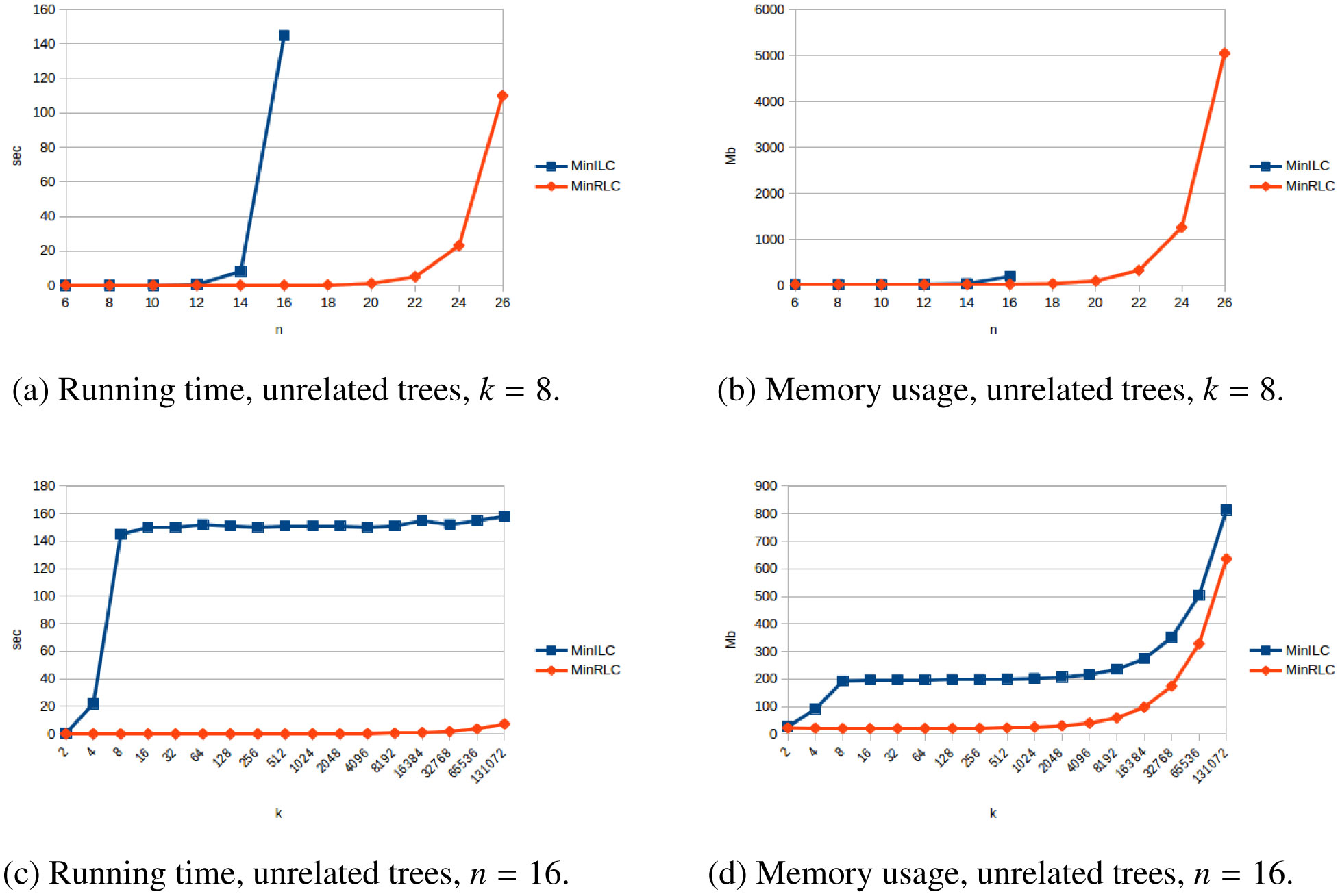
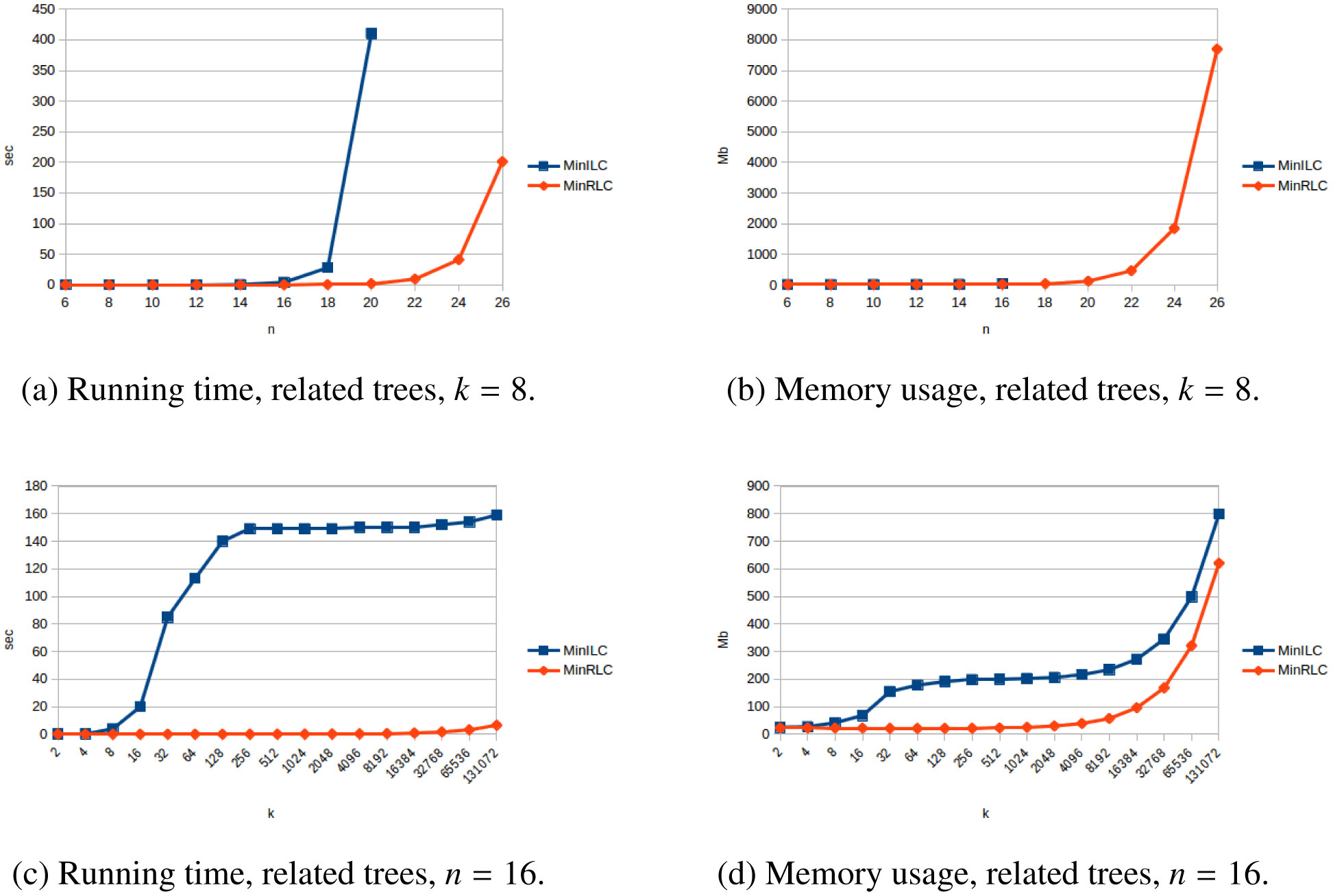
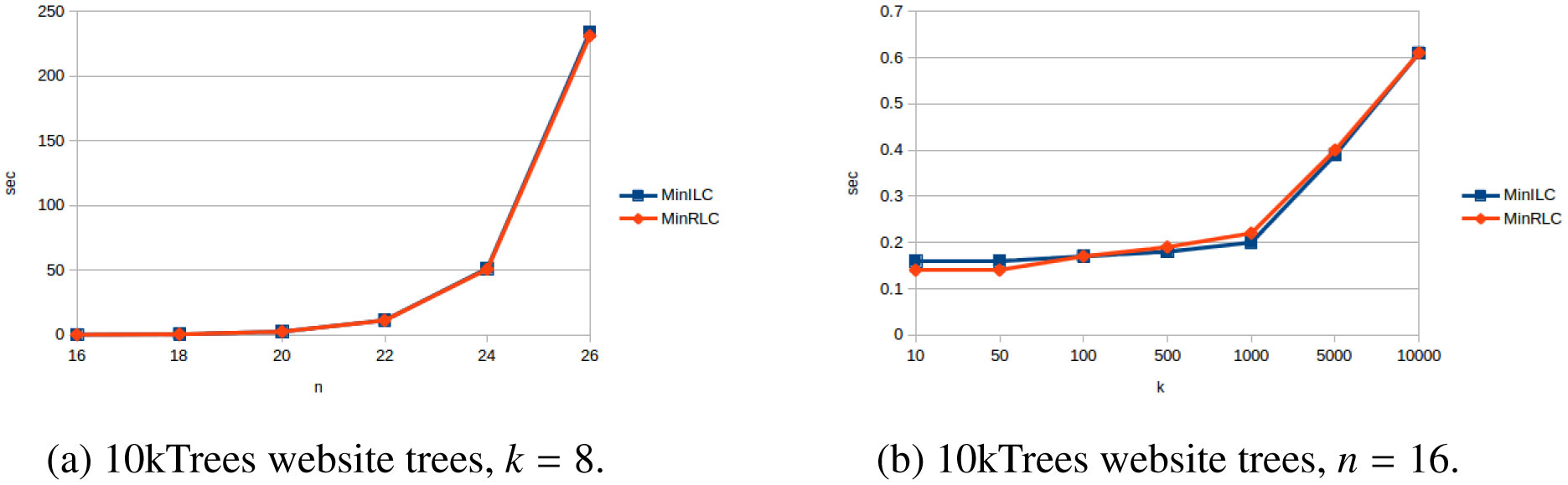
The problem of constructing a minimally resolved phylogenetic supertree (i.e., a rootedtree having the smallest possible number of internal nodes) that contains all of the rooted triplets froma consistent set R is known to be NP-hard. In this article, we prove that constructing a phylogenetictree consistent with R that contains the minimum number of additional rooted triplets is also NP-hard,and develop exact, exponential-time algorithms for both problems. The new algorithms are applied toconstruct two variants of the local consensus tree; for any set S of phylogenetic trees over some leaflabel set L, this gives a minimal phylogenetic tree over L that contains every rooted triplet present in alltrees in S, where “minimal” means either having the smallest possible number of internal nodes or thesmallest possible number of rooted triplets. (The second variant generalizes the RV-II tree, introducedby Kannan et al. in 1998.) We also measure the running times and memory usage in practice of thenew algorithms for various inputs. Finally, we use our implementations to experimentally investigatethe non-optimality of Aho et al.’s well-known BUILD algorithm from 1981 when applied to the localconsensus tree problems considered here.

| [1] |
Adams III EN (1972) Consensus techniques and the comparison of taxonomic trees. Systematic Zoology 21: 390–397. doi: 10.2307/2412432

|
| [2] | Aho AV, Sagiv Y, Szymanski TG, et al. (1981) Inferring a tree from lowest common ancestors with an application to the optimization of relational expressions. SIAM J Comput 10: 405–421. |
| [3] |
Arnold C, Matthews LJ, Nunn CL (2010) The 10kTrees website: A new online resource for primate phylogeny. Evolutionary Anthropology 19: 114–118. doi: 10.1002/evan.20251
|
| [4] | Bender MA, Farach-Colton M (2000) The LCA problem revisited. In Proceedings of the 4thLatin American Symposium on Theoretical Informatics (LATIN 2000), volume 1776 of LNCS, pages 88–94. Springer-Verlag. |
| [5] |
Bininda-Emonds ORP (2004) The evolution of supertrees. TRENDS Ecol Evolution 19: 315–322. doi: 10.1016/j.tree.2004.03.015
|
| [6] |
Bininda-Emonds ORP, Cardillo M, Jones KE, et al. (2007) The delayed rise of present-day mammals. Nature 446: 507–512. doi: 10.1038/nature05634
|
| [7] | Bryant D (1997) Building Trees, Hunting for Trees, and Comparing Trees: Theory and Methods in Phylogenetic Analysis. PhD thesis, University of Canterbury, Christchurch, New Zealand. |
| [8] | Bryant D (2003) A classification of consensus methods for phylogenetics. In Janowitz MF, Lapointe FJ, McMorris FR, et al., editors, Bioconsensus, volume 61 of DIMACS Series in Discrete Mathematics and Theoretical Computer Science, pages 163–184. American Mathematical Society. |
| [9] |
Byrka J, Guillemot S, Jansson J (2010) New results on optimizing rooted triplets consistency. Discrete Applied Mathematics 158: 1136–1147. doi: 10.1016/j.dam.2010.03.004
|
| [10] |
Chor B, Hendy M, Penny D (2007) Analytic solutions for three taxon ML trees with variable rates across sites. Discrete Applied Mathematics 155: 750–758. doi: 10.1016/j.dam.2005.05.043
|
| [11] |
Constantinescu M, Sankoff D (1995) An efficient algorithm for supertrees. J Classification 12: 101–112. doi: 10.1007/BF01202270
|
| [12] | Felsenstein J (2004) Inferring Phylogenies. Sinauer Associates, Inc., Sunderland, Massachusetts. |
| [13] | Garey M, Johnson D (1979) Computers and Intractability – A Guide to the Theory of NPCompleteness. Freeman WH and Company, New York. |
| [14] |
Gąsieniec L, Jansson J, Lingas A, et al. (1999) On the complexity of constructing evolutionary trees. J Combinatorial Optimization 3: 183–197. doi: 10.1023/A:1009833626004
|
| [15] |
He YJ, Huynh TND, Jansson J, et al. (2006) Inferring phylogenetic relationships avoiding forbidden rooted triplets. J Bioinformatics Comput Bio 4: 59–74. doi: 10.1142/S0219720006001709
|
| [16] |
Henzinger MR, King V, Warnow T. (1999) Constructing a tree from homeomorphic subtrees, with applications to computational evolutionary biology. Algorithmica 24: 1–13. doi: 10.1007/PL00009268
|
| [17] | Huson DH, Rupp R, Scornavacca C (2010) Phylogenetic Networks: Concepts, Algorithms and Applications. Cambridge University Press, Cambridge, U.K. |
| [18] |
Jansson J, Lemence RS, Lingas A (2012) The complexity of inferring a minimally resolved phylogenetic supertree. SIAM J Comput 41: 272–291. doi: 10.1137/100811489
|
| [19] | Jansson J, Lingas A, Rajaby R, et al. (2017) Determining the consistency of resolved triplets and fan triplets. In Proceedings of the 21st Annual International Conference on Research in Computational Molecular Biology (RECOMB 2017), volume 10229 of LNCS, pages 82–98. Springer-Verlag. |
| [20] | Jansson J, Rajaby R, Shen C, et al. (to appear). Algorithms for the majority rule (+) consensus tree and the frequency difference consensus tree. IEEE/ACM Transactions Computational Bio Bioinformatics. |
| [21] | Jansson J, Shen C, Sung WK (2016) Improved algorithms for constructing consensus trees. J ACM 63. |
| [22] |
Kannan S,Warnow T, Yooseph S (1998) Computing the local consensus of trees. SIAM J Computing 27: 1695–1724. doi: 10.1137/S0097539795287642
|
| [23] |
McKenzie A, Steel M (2000) Distributions of cherries for two models of trees. Mathematical Biosciences 164: 81–92. doi: 10.1016/S0025-5564(99)00060-7
|
| [24] | Nethercote N, Seward J (2007) Valgrind: a framework for heavyweight dynamic binary instrumentation. In Proceedings of the ACM SIGPLAN 2007 Conference on Programming Language Design and Implementation (PLDI 2007), pages 89–100. ACM. |
| [25] |
Ng MP, Wormald NC (1996) Reconstruction of rooted trees from subtrees. Discrete Applied Mathematics 69: 19–31. doi: 10.1016/0166-218X(95)00074-2
|
| [26] |
Semple C (2003) Reconstructing minimal rooted trees. Discrete Applied Mathematics 127: 489–503. doi: 10.1016/S0166-218X(02)00250-0
|
| [27] |
Semple C, Daniel P, Hordijk W, et al. (2004) Supertree algorithms for ancestral divergence dates and nested taxa. Bioinformatics 20: 2355–2360. doi: 10.1093/bioinformatics/bth246
|
| [28] |
Snir S, Rao S (2006) Using Max Cut to enhance rooted trees consistency. IEEE/ACM Transactions Comput Bio Bioinformatics 3: 323–333. doi: 10.1109/TCBB.2006.58
|
| [29] |
Steel M (1992) The complexity of reconstructing trees from qualitative characters and subtrees. J Classification 9: 91–116. doi: 10.1007/BF02618470
|
| [30] | Sung WK (2010) Algorithms in Bioinformatics: A Practical Introduction. Chapman & Hall/CRC, Boca Raton, Florida. |
| [31] |
Willson SJ. (2004) Constructing rooted supertrees using distances. Bulletin Mathematical Bio 66: 1755–1783. doi: 10.1016/j.bulm.2004.04.006
|
| [32] | Wulff-Nilsen C (2013) Faster deterministic fully-dynamic graph connectivity. In Proceedings of the 24th Annual ACM-SIAM Symposium on Discrete Algorithms (SODA 2013), pages 1757–1769. SIAM. |
Figures(11) / Tables(5)

Jesper Jansson, Ramesh Rajaby, Wing-Kin Sung. Minimal Phylogenetic Supertrees and Local Consensus Trees[J]. AIMS Medical Science, 2018, 5(2): 181-203. doi: 10.3934/medsci.2018.2.181


 DownLoad: