Salmon calcitonin: conformational changes and stabilizer effects

Shan-Yang Lin; Shan-Yang Lin

doi:10.3934/biophy.2015.4.695

AIMS Biophysics

2015, Volume 2, Issue 4: 695-723. doi: 10.3934/biophy.2015.4.695

Previous Article Next Article

Review Topical Sections

Salmon calcitonin: conformational changes and stabilizer effects

Shan-Yang Lin ^,

Laboratory of Pharmaceutics & Biopharmaceutics, Department of Biotechnology and Pharmaceutical Technology, Yuanpei University, Hsin Chu 30015, Taiwan, ROC

Received: 03 October 2015 Accepted: 09 November 2015 Published: 11 November 2015

The therapeutic activity of peptides or protein drugs is highly dependent on their conformational structure. The protein structure is flexible and responds to external conditions, which may compromise the protein's native conformation and influence its physical and chemical stability. The physical and chemical stability of peptides or protein drugs are important characteristics of biopharmaceutical products. Calcitonin (CT) is a polypeptide hormone that participates in diverse physiological functions in humans; therefore, it is a potentially useful protein for investigations of different aspects of pharmacology and drug delivery systems. Of the different types of CT available for clinical use, salmon CT (sCT) is one of the most potent. In this review article, the commercially available sCT was selected as a suitable peptide candidate for the discussion of its stability and conformational changes in the aqueous and solid states using Fourier transform infrared (FTIR) spectroscopic analysis under different external conditions, including pH, temperature, drying method, and added excipients. Particularly, excipients that have been optimized as stabilizers of sCT in aqueous solution and as lyophilized and spray-dried drug formulations are also discussed.

Keywords:

Citation: Shan-Yang Lin. Salmon calcitonin: conformational changes and stabilizer effects[J]. AIMS Biophysics, 2015, 2(4): 695-723. doi: 10.3934/biophy.2015.4.695

Related Papers:

[1]	Li-Bin Liu, Yige Liao, Guangqing Long . Error estimate of BDF2 scheme on a Bakhvalov-type mesh for a singularly perturbed Volterra integro-differential equation. Networks and Heterogeneous Media, 2023, 18(2): 547-561. doi: 10.3934/nhm.2023023
[2]	Xiongfa Mai, Ciwen Zhu, Libin Liu . An adaptive grid method for a singularly perturbed convection-diffusion equation with a discontinuous convection coefficient. Networks and Heterogeneous Media, 2023, 18(4): 1528-1538. doi: 10.3934/nhm.2023067
[3]	Li-Bin Liu, Limin Ye, Xiaobing Bao, Yong Zhang . A second order numerical method for a Volterra integro-differential equation with a weakly singular kernel. Networks and Heterogeneous Media, 2024, 19(2): 740-752. doi: 10.3934/nhm.2024033
[4]	Dilip Sarkar, Shridhar Kumar, Pratibhamoy Das, Higinio Ramos . Higher-order convergence analysis for interior and boundary layers in a semi-linear reaction-diffusion system networked by a $ k $-star graph with non-smooth source terms. Networks and Heterogeneous Media, 2024, 19(3): 1085-1115. doi: 10.3934/nhm.2024048
[5]	Chaoqun Huang, Nung Kwan Yip . Singular perturbation and bifurcation of diffuse transition layers in inhomogeneous media, part II. Networks and Heterogeneous Media, 2015, 10(4): 897-948. doi: 10.3934/nhm.2015.10.897
[6]	Yongqiang Zhao, Yanbin Tang . Approximation of solutions to integro-differential time fractional wave equations in $ L^{p}- $space. Networks and Heterogeneous Media, 2023, 18(3): 1024-1058. doi: 10.3934/nhm.2023045
[7]	Chaoqun Huang, Nung Kwan Yip . Singular perturbation and bifurcation of diffuse transition layers in inhomogeneous media, part I. Networks and Heterogeneous Media, 2013, 8(4): 1009-1034. doi: 10.3934/nhm.2013.8.1009
[8]	Gianni Dal Maso, Francesco Solombrino . Quasistatic evolution for Cam-Clay plasticity: The spatially homogeneous case. Networks and Heterogeneous Media, 2010, 5(1): 97-132. doi: 10.3934/nhm.2010.5.97
[9]	Ciro D’Apice, Umberto De Maio, T. A. Mel'nyk . Asymptotic analysis of a perturbed parabolic problem in a thick junction of type 3:2:2. Networks and Heterogeneous Media, 2007, 2(2): 255-277. doi: 10.3934/nhm.2007.2.255
[10]	Rémi Goudey . A periodic homogenization problem with defects rare at infinity. Networks and Heterogeneous Media, 2022, 17(4): 547-592. doi: 10.3934/nhm.2022014

Abstract

1. Introduction

Consider the following singularly perturbed Fredholm integro-differential equation (SPFIDE) in the interval $ \bar{I} = [0, T] $:

$\begin{equation} \left\{ \begin{aligned}&Lu\left ( t \right ): = \varepsilon{u}'\left ( t \right )+f\left ( t, u\left ( t \right ) \right )+\lambda \int_{0}^{T}K\left ( t, s, u\left ( s \right ) \right )ds = 0, \ t\in I = \left ( 0, T \right ], \\ &u\left ( 0 \right ) = A, \end{aligned}\right. \end{equation}$ $

(1.1)

where $ 0 < \varepsilon \ll 1 $ is a perturbation parameter, $ A $ is a given constant and $ \lambda $ is a real parameter. We assume that $ f\left (t, u \right)\in C^1\left(\bar{I}\times R\right) $, $ K\left (t, s, u \right)\in C^1\left(\bar{I}\times\bar{I}\times R\right) $ and there exist constants $ \alpha $, $ \beta $ such that $ 0 < \alpha\le\left | \partial f/\partial u \right | $, $ \left | \partial K/\partial u \right |\leq \beta $. Under these assumptions, the problem (1.1) has a unique solution (see ^[1]).

It is well known that the SPFIDEs arise widely in scientific fields such as mathematical biology ^[2], material mechanics ^[3], hydrodynamic ^[4] and so on.These problems depend on such a small positive parameter $ \varepsilon $ that the solution varies rapidly when $ \varepsilon \rightarrow 0 $. Due to the presence of this perturbation parameter $ \varepsilon $, classical numerical methods on a uniform mesh fail to give accurate results. Therefore, it is necessary to develop suitable numerical methods that are $ \varepsilon $-uniformly convergent for solving these problems.

Over the past few years, there has been a growing interest in the numerical methods for Volterra integro-differential equations (see, e.g., ^{[5,6,7,8,9,10]}) and Fredholm integro-differential equations (see, e.g., ^[11,12]). When the differential term of these integro-differential equations contains a small positive perturbation parameter $ \varepsilon $, these problems are called singularly perturbed integro-differential equations. Recently, some robust numerical methods are proposed to solve singularly perturbed Volterra integro-differential equations^{[13,14,15,16]}. Meanwhile, the authors in ^[17,18] developed fitted finite difference schemes on a uniform mesh for second-order SPFIDEs and gave some convergence results based on the prior information of the exact solution. Durmaz, et.al., ^[19] proposed a second-order uniformly convergent finite difference scheme on a Shishkin mesh for a singularly perturbed Fredholm integro-differential equation with the reduced second type Fredholm equation. In ^[20], the authors presented a fitted finite difference approach on a Shishkin mesh for a first-order singularly perturbed Fredholm integro-differential initial value problem with integral condition. Kumar et al. ^[21] proposed a non-standard finite difference scheme with Haar wavelet basis functions for a singularly perturbed partial integro-differential equation. Recently, Cakir et al., ^[22] solved first-order nonlinear SPFIDEs on a Sinshkin mesh with first-order convergence rate.

From the literatures we have mentioned above, the existing numerical methods of SPFIDEs given in ^[19,20,21] are layer-adapted mesh approaches, which require a priori information about the location and width of the boundary layer. Thus, adaptive grid methods by equidistributing monitor functions are widely used to solve some singularly perturbed problems, see ^{[25,26,27,28,29]} for example. The advantages of these adaptive grid methods is to cluster automatically the grid points within the boundary layer. To the best of our knowledge, there is no report about this adaptive grid method for problem (1.1). Therefore, the aim of this paper is to solve problem (1.1) numerically by a finite difference scheme on an adaptive grid obtained by equidistributing a positive monitor function. The discrete scheme is constructed by using the backward Euler formula and right rectangle formula to approximate derivative term and nonlinear integral term, respectively. It is proved under some additional conditions that the proposed adaptive grid method is first-order uniformly convergent, with respect to $ \varepsilon $.

The rest of this paper is as follows. In Section 2, preliminary results of the exact solution are laid out. A discretization scheme is established in Section 3, in which a prior error analysis and a posterior error estimate are carried out successively. Numerical results obtained by the adaptive gird algorithm are given in Section 4 to support the theoretical analyses. The paper ends with a summary of the main conclusions in Section 5.

Notation Throughout this paper, $ C $ which is not necessarily the same at each occurrence, indicates a positive constant independent of the mesh division parameter $ N $ or the singular perturbation parameter $ \varepsilon $. To simplify the notation, we set $ v_{k} = v\left (t_{k} \right) $ for any function $ v(t) $. In our estimates, the maximum norm of a continuous function $ v(t) $ with the domain $ [0, T] $ is defined as $ \left \| v\left (t \right) \right \|_{\infty} = \mathrm{ess} \underset{t\in \left [0, T \right]}{\sup} \left | v\left (t \right) \right | $ as well as the maximum norm of a discrete vector $ \mathit{\boldsymbol{x}} = \left \{ x_i \right \}_{i = 0}^{N} $ with $ N+1 $ elements is defined as $ \left \| \mathit{\boldsymbol{x}} \right \|_{\infty} = \underset{i = 0, 1, 2, \cdots, N}{\max }\left | x_{i} \right | $.

2. Preliminary results

In this section, we list the bounds for the exact solution $ u\left(t\right) $ and its first-order derivative.

Lemma 2.1. [22, Lemma 1] Assume the constant $ \lambda $ satisfies

$\begin{equation} \left | \lambda \right | < \frac{\alpha }{\underset{0\leq t\leq T}{\max}\int_{0}^{T}\left | G\left ( t, s \right ) \right |ds}. \end{equation}$ $

(2.1)

Then we have

$\begin{eqnarray} &&\left \| u \right \| _{\infty } \le C_{0}, \end{eqnarray}$ $

(2.2)

$\begin{eqnarray} && \left | u'\left(t\right) \right |\le C\left ( 1+\frac{1}{\varepsilon}e^{-\frac{\alpha t}{\varepsilon}} \right ) , \ 0\le t\le T, \end{eqnarray}$ $

(2.3)

where

$\begin{eqnarray*} &&C_{0} = \frac{\left | A \right |+\frac{1}{\alpha}\left \|q\right \|_{\infty}}{1-\frac{1}{\alpha}\left | \lambda \right |\underset{0\leq t\leq T}{\max}\int_{0}^{T}\left | G\left ( t, s \right ) \right |ds}, \\ &&G\left(t, s\right) = \frac{\partial }{\partial u} K\left(t, s, \gamma u\right), \ 0 < \gamma < 1, \\ &&q\left(t\right) = -f\left(t, 0\right)-\gamma \int_{0}^{T} K\left(t, s, 0\right)ds. \end{eqnarray*}$ $

Corollary 2.1. For any two functions $ v\left(t\right) $ and $ w\left(t\right) $ satisfying

$\begin{equation} v\left(0\right) = w\left(0\right) = A, \ \end{equation}$ $

(2.4)

and

$\begin{equation} Lv\left(t\right)-Lw\left(t\right) = \tilde{F}\left(t\right), \ t\in I, \ \end{equation}$ $

(2.5)

where $ \tilde{F}(t) $ is a bounded piece-wise continuous function, we have

$\begin{equation} \left \| v\left(t\right)-w\left(t\right) \right \|_{\infty}\le C\left \| Lv\left(t\right)-Lw\left(t\right) \right \|_{\infty}.\ \end{equation}$ $

(2.6)

Proof. The proof is similar to [15, Corollary 2.1].

3. Discretization and error analysis

3.1. Discrete scheme

Let $ \bar{\Omega } _{N}: = \left\{0 = t_{0} < t_{1} < \dots < t_{N} = T \right\} $ be an arbitrary non-uniform mesh and $ h_{i} = t_{i}-t_{i-1} $ be the local mesh size for $ i = 1, 2, \cdots, N $. For a given mesh function $ \left \{ v_{i} \right \} _{i = 0}^{N} $, define the backward finite difference operator as follows:

$\begin{equation} D^-v_i = \frac{v_i-v_{i-1}}{h_i}, \ i = 1, 2, \cdots, N. \end{equation}$ $

(3.1)

Then to construct the discretization scheme for problem (1.1), we integrate Eq (1.1) over $ \left(t_{i-1}, t_i \right) $ and use the right rectangle rule to approximate the integral part, which yield,

$\begin{equation} \left\{ \begin{aligned} &\varepsilon D^{-}u_{i}+f\left(t_i, u_i\right)+\lambda \sum\limits_{j = 1}^{N}h_jK\left(t_i, t_j, u_j\right)+R_i = 0, \ i = 1, 2, \cdots, N, \\ &u_0 = A, \end{aligned} \right. \end{equation}$ $

(3.2)

where

$\begin{equation} R_i: = R_i^{\left(1\right)}+R_i^{\left(2\right)}+R_i^{\left(3\right)} \end{equation}$ $

(3.3)

and

$\begin{eqnarray*} && R_i^{\left(1\right)} = -h_i^{-1}\int_{t_{i-1}}^{t_i}(t-t_{i-1})\frac{d }{d t} f\left(t, u\left(t\right)\right)dt, \\ &&R_i^{\left(2\right)} = -\lambda h_i^{-1}\int_{t_{i-1}}^{t_i}\left(t-t_{i-1}\right)\int_0^T\frac{\partial }{\partial t} K\left(t, s, u\left(s\right)\right)dsdt, \\ && R_i^{\left(3\right)} = -\lambda \sum\limits_{j = 1}^{N}\int_{t_{j-1}}^{t_j}\left(s-t_{j-1}\right)\frac{d }{d s} K\left(t_i, s, u\left(s\right)\right)ds.\ \end{eqnarray*}$ $

Neglecting the truncation error $ R_i $ in Eq (3.2), we obtain the discretization scheme of problem (1.1)

$\begin{equation} \left\{ \begin{aligned}&L^Nu_i^N: = \varepsilon D^-u_i^N+f\left(t_i, u_i^N\right)+\lambda\sum\limits_{j = 1}^{N}h_jK\left(t_i, t_j, u_j^N\right) = 0, \ i = 1, 2, \cdots, N, \\ &u_0 = A, \end{aligned}\right. \end{equation}$ $

(3.4)

where $ u_i^N $ is the approximation of $ u(t) $ at point $ t = t_i $.

3.2. A prior error analysis

Let $ e_i^N: = u_i^N-u_i $, $ i = 0, 1, \cdots, N $, be the absolute error at $ t_i $ of the numerical solution. Then we can obtain the following error equations

$\begin{equation} \left\{ \begin{aligned} &L^Nu_i^N-L^Nu_i = R_i, \ i = 1, 2, \cdots, N, \\ &e_0^N = 0, \end{aligned}\right. \end{equation}$ $

(3.5)

where $ R_i $ is the local truncation error defined in Eq (3.3) at $ t_i $.

Lemma 3.1. For $ i = 1, 2, \cdots, N $, the truncation error $ R_i $ defined in Eq (3.3) satisfies

$\begin{equation} \left | R_i \right | \le C\max\limits_{1\le i\le N} \int_{t_{i-1}}^{t_i}\left(1+\left | {u}'\left(t\right) \right |\right)dt. \ \end{equation}$ $

(3.6)

Proof. At first, based on the conditions $ f\left(t, u\right)\in C^1(\bar{I}\times R) $ and $ 0 < \alpha\le\left | \partial f/\partial u \right | $, we obtain

$\begin{equation} \begin{aligned} \left | R_i^{\left(1\right)} \right |& \le h_{i}^{-1}\int_{t_{i-1}}^{t_i}h_i \left(\left | \frac{\partial f\left(t, u\right)}{\partial t} \right |+\left | \frac{\partial f\left(t, u\right)}{\partial u} \right | \left | u'\left(t\right) \right | \right)dt\\ &\le C\int_{ t_{i-1}}^{t_i}\left(1+\left | u'\left(t\right) \right |\right)dt.\ \end{aligned} \end{equation}$ $

(3.7)

Then, since $ K\left(t, s, u\right)\in C^1\left(\bar{I}\times\bar{I}\times R\right) $ and $ \left | \partial K /\partial u \right | \le \beta $, we have

$\begin{equation} \begin{aligned} \left | R_i^{\left(2\right)} \right | &\le\left | \lambda \right | \int_{t_{i-1}}^{t_i} \int_{0}^{T}\left | \frac{\partial }{\partial t}K\left(t, s, u\left(s\right)\right) \right |dsdt\\ & \le Ch_i.\ \end{aligned} \end{equation}$ $

(3.8)

and

$\begin{equation} \begin{aligned} \left | R_i^{\left(3\right)} \right |&\le \left | \lambda \right | \sum\limits_{j = 1}^{N}T \int_{t_{j-1}}^{t_j}\left(\left | \frac{\partial K\left(t_i, s, u\right)}{\partial s} \right | +\left | \frac{\partial K\left(t_i, s, u\right)}{\partial u} \right |\left | u'\left(s\right) \right | \right)ds \\ &\le C\max\limits_{1\le j\le N}\int_{t_{j-1}}^{t_j}\left(1+\left | u'\left(t\right) \right |\right) dt.\ \end{aligned} \end{equation}$ $

(3.9)

Finally, the desired result of this lemma can be followed by Eqs (3.7), (3.8) and (3.9).

Lemma 3.2. Under the assumption

$\begin{equation} \left | \lambda \right | < \frac{1}{\alpha}\max\limits_{1\le i\le N}\sum\limits_{j = 1}^{N}h_j\left | G_{ij} \right |, \ \end{equation}$ $

(3.10)

we have

$\begin{equation} \left \| \mathit{\boldsymbol{e}}^N \right \| _{\infty}\le \frac{1}{\alpha}\left(1-\frac{1}{\alpha}\left | \lambda \right |\max\limits_{1\le i\le N}\sum\limits_{j = 1}^{N}h_i\left | G_{ij} \right | \right)^{-1}\left \|\mathit{\boldsymbol{R}} \right \|_{\infty}, \ \end{equation}$ $

(3.11)

where $ \mathit{\boldsymbol{e}}^N = \left \{ e_i^N \right \} _{i = 0}^{N} $, $ \mathit{\boldsymbol{R}} = \left \{ R_i \right \} _{i = 0}^{N} $ and $ G_{ij} = \frac{\partial }{\partial u}K\left(t_i, s_j, u_j+\zeta e_j^N\right), \ 0 < \zeta < 1 $.

Proof. Applying the mean value theorem to Eq (3.5), we get

$\begin{equation} \varepsilon D^-e_i^N+a_ie_i^N+\lambda \sum\limits_{j = 1}^{N}h_jG_{ij}e_j^N = R_i, \ i = 1, 2, \cdots, N, \end{equation}$ $

(3.12)

where

$\begin{eqnarray} &&a_i = \frac{\partial }{\partial u}f\left(t_i, u_i+\xi e_i^N\right), \ 0 < \xi < 1, \end{eqnarray}$ $

(3.13)

$\begin{eqnarray} &&G_{ij} = \frac{\partial }{\partial u}K\left(t_i, s_j, u_j+\zeta e_j^N\right), \ 0 < \zeta < 1 . \end{eqnarray}$ $

(3.14)

According to maximum principle for the operator $ \varepsilon D^-e_i^N+a_ie_i^N $, we have

$\begin{equation} \left \| \mathit{\boldsymbol{e}}^N \right \| _\infty \le \frac{1}{\alpha}\left \| \mathit{\boldsymbol{R}} \right \| _\infty +\frac{1}{\alpha}\left | \lambda \right | \left \| \mathit{\boldsymbol{e}}^N \right \| _\infty \max\limits_{1\le i\le N}\sum\limits_{j = 1}^{N}h_j\left | G_{ij} \right |, \end{equation}$ $

(3.15)

which immediately leads to the desired result with the assumption (3.10).

Based on the above Lemmas 3.1–3.2, we get the following convergence results.

Theorem 3.1. Let $ u(t) $ be the solution of problem (1.1) and $ u_i^N $ be the solution of discrete scheme (3.4). Then

$\begin{equation} \max\limits_{1\le i\le N}\left | u_i^N-u_i \right | \le C \max\limits_{1\le i\le N}\int_{t_{i-1}}^{t_i}\left(1+\left | {u}'\left(t\right) \right |\right)dt. \end{equation}$ $

(3.16)

Corollary 3.1. Under the conditions of Theorem 3.1, there exists an adaptive grid $ \left \{ t_i \right \} _{i = 0}^{N} $ such that

$\begin{equation} \max\limits_{1\le i\le N}\left | u_i^N-u_i \right |\le CN^{-1}. \ \end{equation}$ $

(3.17)

Proof. Based on the mesh equidistribution principle presented in ^[29], the mesh $ \left \{ t_i \right \}_{i = 0}^{N} $ given by our adaptive grid algorithm satisfies

$\begin{equation} \int_{t_{i-1}}^{t_i}M\left(t\right)dt = \frac{1}{N}\int_{0}^{T}M\left(t\right)dt, \ i = 1, 2, \cdots, N, \end{equation}$ $

(3.18)

where $ M(t) $ is called the monitor function, which can be chosen as

$\begin{equation} M\left(t\right) = 1+\left | {u}'\left(t\right) \right |.\ \end{equation}$ $

(3.19)

Therefore, it follows from Lemma 2.1 that

$\begin{equation} \begin{aligned} \max\limits_{1\le i\le N}\left | u_i^N-u_i \right | &\le C \max\limits_{1\le i\le N}\int_{t_{i-1}}^{t_i}\left(1+\left | {u}'\left(t\right) \right |\right)dt\\ & = \frac{C}{N}\int_{0}^{T}\left(1+\left | {u}'\left(t\right) \right | \right)dt\\ &\le \frac{C}{N}\int_{0}^{T}\left(1+\frac{1}{\varepsilon }\exp\left(-\frac{\alpha t}{\varepsilon } \right)\right)dt\\ &\le \frac{C}{N}\left(T+\frac{1}{\alpha}\left(1-\exp\left(-\frac{\alpha T}{\varepsilon } \right)\right)\right)\\ &\le\frac{C}{N}. \end{aligned} \end{equation}$ $

(3.20)

3.3. A posteriori error analysis

In this section, we shall derive an a posteriori error estimation for the numerical solution $ \left \{ u_i^N \right \} _{i = 0}^{N} $. Recall that $ \tilde{u}^N\left(t\right) $ is a piece-wise linear interpolation function through knots $ \left(t_i, u_i^N\right), \ i = 0, 1, \cdots, N $. Then, for any $ t\in J_i: = \left [t_{i-1}, t_i \right] $, we obtain

$\begin{equation} \tilde{u}^N\left(t\right) = u_i^N+D^-u_i^N\left(t-t_i\right), \ i = 1, 2, \cdots, N.\ \end{equation}$ $

(3.21)

Theorem 3.2. Let $ u(t) $ be the exact solution of problem (1.1), $ \left \{ u_i^N \right \} _{i = 0}^{N} $ be the discrete solution of problem (3.4) and $ \tilde{u}^N(t) $ be its piece-wise linear interpolation function defined in Eq (3.21). Then we have

$\begin{equation} \left \| \tilde{u}^N\left(t\right)-u\left(t\right) \right \|_{\infty}\le C \max\limits_{1\le i\le N}\left(h_i+h_i\left | D^-u_i^N \right | \right).\ \end{equation}$ $

(3.22)

Proof. For any $ t\in\left (t_{i-1}, t_i \right] $, it follows from Eq (1.1) and Eq (3.4) that

$\begin{equation} \begin{aligned} L\tilde{u}^N\left(t\right)-Lu\left(t\right) & = \varepsilon D^-u_i^N+f\left(t, \tilde{u}^N\left(t\right)\right)+\lambda \int_0^TK\left(t, s, \tilde{u}^N\left(s\right)\right)ds\\ & = -f\left(t_i, u_i^N\right)-\lambda \sum\limits_{j = i}^{N}h_jK\left(t_i, t_j, u_j^N\right) \\ &\quad +f\left(t, \tilde{u}^N\left(t\right)\right)+\lambda \int_0^TK\left(t, s, \tilde{u}^N\left(s\right)\right)ds\\ & = P\left(t\right)+Q\left(t\right), \ \end{aligned} \end{equation}$ $

(3.23)

where

$\begin{eqnarray} &&P\left(t\right) = f\left(t, \tilde{u}^N\left(t\right)\right)-f\left(t_i, u_i^N\right), \end{eqnarray}$ $

(3.24)

$\begin{eqnarray} && Q\left(t\right) = \lambda \int_{0}^{T}K(t, s, \tilde{u}^N\left(s)\right)ds-\lambda \sum\limits_{j = 1}^{N}h_jK\left(t_i, t_j, u_j^N\right) . \end{eqnarray}$ $

(3.25)

With the assumptions of functions $ f\left(t, u\right) $, $ K\left(t, s, u\right) $ and the definition of $ \tilde{u}^N\left(t\right) $, we have

$\begin{equation} \begin{aligned} \left | P\left(t\right) \right | & = \left | f\left(t_i, u_i^N\right)+\int_{t_i}^{t}\frac{df\left(\tau, \tilde{u}^N\left(\tau\right)\right)}{d\tau}d\tau-f\left(t_i, u_i^N\right) \right | \\ &\le \int_{t}^{t_i}\left(\left | \frac{\partial f\left(\tau, \tilde{u}^N\right)}{\partial \tau} \right |+ \left | \frac{\partial f\left(\tau, \tilde{u}^N\right)}{\partial u} \right |\left | D^-u_i^N \right |\right) d\tau \\ &\le C h_i\left(1+\left | D^-u_i^N \right |\right) \end{aligned} \end{equation}$ $

(3.26)

and

$\begin{equation} \begin{aligned} \left | Q\left(t\right) \right |& = \left | \lambda \sum\limits_{j = 1}^{N}\int_{t_{j-1}}^{t_j}\left(K\left(t, s, \tilde{u}^N\left(s\right)\right)-K\left(t_i, t_j, u_j^N\right)\right)ds \right | \\ &\le\left |\lambda\right | \sum\limits_{j = 1}^{N} \int_{t_{j-1}}^{t_j}\left(\left |\frac{\partial }{\partial t} K\left(\xi_1t+\left(1-\xi_1\right)t_i, s, \tilde{u}^N\left(s\right)\right)\left(t-t_{i}\right)\right |\right.\\ &\quad+\left |\frac{\partial }{\partial s} K\left(t_i, \xi_2s+\left(1-\xi_2\right)t_{j}, \tilde{u}^N\left(s\right)\right)\left(s-t_{j}\right)\right |\\ &\left. \quad+\left | \frac{\partial }{\partial u}K\left(t_i, t_{j}, \xi_3\tilde{u}^N\left(s\right)+\left(1-\xi_3\right)u_{j}^N\right)\left(\tilde{u}^N\left(s\right)-u_{j }^N\right)\right |\right) ds\\ &\le C\left(h_i+\max\limits_{1\le j\le N} h_j \left(1+\left | D^-u_j^N \right |\right)\right), \ \end{aligned} \end{equation}$ $

(3.27)

where $ 0 < \xi_1 < 1 $, $ 0 < \xi_2 < 1 $, and $ 0 < \xi_3 < 1 $. The result can be derived from Eqs (3.23), (3.26), (3.27) and Corollary 2.1.

From Corollary 3.1, it is easy to conclude that there exists a mesh $ \left \{ t_i \right \}_{i = 0}^{N} $ and a monitor function $ M\left(t\right) $ given in Eq (3.19) such that the inequality (3.17) holds true. However, $ {u}'\left(t\right) $ is not available. Therefore, based on the a posterior error estimation (3.22), we choose the discrete analogue of $ M\left(t\right) $ as

$\begin{equation} {\tilde{M}_i = 1+\left | D^-u_i^N \right |, i = 1, 2, \cdots, N.\ } \end{equation}$ $

(3.28)

Therefore, the idea is to adaptively design a mesh in which the values of monitor function $ tilde{M}_i $ are the same on each mesh interval. This is equivalent to find $ \left \{ \left(t_i, u_i^N\right) \right \}_{i = 0}^{N} $, such that

$\begin{equation} h_i\tilde{M}_i = \frac{1}{N}\sum\limits_{j = 1}^{N}h_j\tilde{M}_j, \ i = 1, 2, \cdots, N.\ \end{equation}$ $

(3.29)

Furthermore, to obtain this equidistributed mesh $ \left\{t_i\right\}_{i = 0}^N $ and the corresponding numerical solution $ u_i^N $, we give the following iteration algorithm:

Algorithm 1 Steps of adaptive grid algorithm

1: Step 1: For a given $ N $, let $ \{t_i^{(0)}\} _{i = 0}^{N} $ be an initial mesh with mesh step $ \frac{1}{N} $. Choose a constant $ \mu^{*} > 1 $ that controls when the algorithm terminates.
2: Step 2: For a given mesh $ \{t_i^{(k)}\}_{i = 0}^{N} $ and numerical solution $ \{u_i^{N, (k)}\}_{i = 0}^{N} $, compute $ \tilde{M}_i^{(k)}, i = 1, 2, \cdots, N $ in Eq (3.28) and set $ \tilde{M}_0^{(k)} = 0 $.
3: Step 3: Set $ h_i^{(k)} = t_i^{(k)}-t_{i-1}^{(k)} $ for each $ i $ and set $ L_0^{(k)} = 0 $ and $ L_i^{(k)} = \sum_{j = 1}^{i}h_j^{(k)}\tilde{M}_j^{(k)} $ for $ i = 1, 2, \cdots, N $. Define
$

$\begin{array}{*{20}{c}} {\mu^{(k)}: = \frac{N}{L_N^{(k)}}\max\limits_{i = 0, 1, \cdots, N}h_i^{(k)}\tilde{M}_i^{(k)}.} & {} & {} & {} & {(3.30)} \end{array}$ $
4: Step 4: Set $ Y_i^{(k)} = iL_N^{(k)}/N $ for $ i = 0, 1, \cdots, N $. Interpolate (see [30, Remark 5.1]) to the points $ (L_i^{(k)}, t_i^{(k)}) $. Generate the new mesh $ \{t_i^{(k+1)}\}_{i = 0}^{N} $ by evaluating this interpolant at the $ Y_i^{(k)} $ for $ i = 0, 1, \cdots, N $.
5: Step 5: If $ \mu^{(k)}\leq\mu^* $, then take $ \{t_i^{(k+1)}\}_{i = 0}^{N} $ as the final mesh and compute $ \{u_i^{N, (k+1)}\}_{i = 0}^{N} $. Otherwise return to Step 2.

4. Numerical experiments and discussion

In Section 4.1, We first present the iterative scheme. Then numerical experiments are given in Section 4.2 to validate the theoretical result of this paper. All experiments were performed on a Windows 10 (64 bit) PC-Intel(R) Core(TM) i5-4200H CPU 2.80 GHz, 8 GB of RAM using MATLAB R2021a.

4.1. Iterative scheme

In order to avoid solving the nonlinear equations (3.4), we apply the quasilinearization technique that performs a first-order Taylor expansion on the last iteration values and obtain

$\begin{equation} \left\{ \begin{aligned}&u_{i}^{N, \left(k\right)} = \frac{\varepsilon /h_i u_{i-1}^{N, \left(k\right)}+B_iu_i^{N, \left(k-1\right)}+C_i }{\varepsilon/h_i +B_i }, i = 1, 2, \cdots, N, \\ &u_0^{N, \left(k\right)} = A, \end{aligned} \right. \end{equation}$ $

(4.1)

where

$\begin{eqnarray} &&B_i = \frac{\partial }{\partial u} f\left(t_i, u_i^{N, \left(k-1\right)}\right), \end{eqnarray}$ $

(4.2)

$\begin{eqnarray} &&C_i = -f\left(t_i, u_{i}^{N, \left(k-1\right)}\right)-\lambda \sum\limits_{j = 1}^{N}h_jK\left(t_i, t_j, u_j^{N, \left(k-1\right)}\right). \end{eqnarray}$ $

(4.3)

4.2. Numerical examples

For all the numerical experiments below, we choose $ \mu^* = 1.1 $, which is defined in Step 4 in Algorithm 1.

Example 4.1. We consider a SPFIDE in the form ^[22]

$\begin{equation} \left\{ \begin{aligned} &\varepsilon {u}'\left(t\right)+2u\left(t\right)+\tanh \left(u\left(t\right)\right)-e^t+\frac{1}{4}\int_{0}^{1}t^2\sin \left(u\left(s\right)\right)ds = 0, \ t\in\left(0, 1\right], \\ &u(0) = 1. \end{aligned} \right. \end{equation}$ $

(4.4)

Since the analytic solution of this problem is not available, we use the following formulas to calculate the errors and the corresponding convergence rates:

$\begin{equation} e_{\varepsilon }^N = \left \| \hat{\mathit{\boldsymbol{u}}}^{2N}-\mathit{\boldsymbol{u}}^N \right \| _{\infty}, \ p_{\varepsilon }^N = \log_{2}{\left(\frac{e_{\varepsilon }^{N} }{e_{\varepsilon }^{2N} } \right)} , \ \end{equation}$ $

(4.5)

where $ \hat{\mathit{\boldsymbol{u}}}^{2N} $ is the numerical solution obtained on the fine mesh $ \bar{\Omega } _{2N} = \bar{\Omega } _{N}\bigcup \left\{\frac{t_{i}+t_{i+1}}{2}\right\}_{i = 0}^{N-1} $. The maximum errors and $ \varepsilon $-uniform rates of the convergence are respectively defined as

$\begin{equation} e^N = \max\limits_\varepsilon e^N_\varepsilon, \ p^N = \log_{2}{\left(\frac{e^{N}}{e^{2N}}\right)}. \end{equation}$ $

(4.6)

In the numerical experiments, we apply the presented adaptive grid algorithm to solve this problem. The resulting errors $ e_{\varepsilon }^N $ and the orders of the convergence $ p_{\varepsilon }^N $, for particular values of $ \varepsilon $ and $ N $ are listed in Table 1. In addition, to compare the performance of the presented adaptive mesh with the Shishkin mesh ^[22] and the Bakhvalov mesh ^[23], some numerical results are given in Table 2.

Table 1. The errors and corresponding convergence rates for Example 4.1.

$ \varepsilon $	$ N=64 $	$ N=128 $	$ N=256 $	$ N=512 $	$ N=1024 $
$ 2^{-2} $	0.004663	0.002384	0.001222	0.000619	0.000312
	0.9680	0.9637	0.9811	0.9903	-
$ 2^{-4} $	0.00595	0.003152	0.00163	0.000801	0.000412
	0.9167	0.9515	1.0244	0.9610	-
$ 2^{-6} $	0.006539	0.003482	0.001818	0.000939	0.000477
	0.9089	0.9373	0.9532	0.9769	-
$ 2^{-8} $	0.006711	0.003633	0.001893	0.000979	0.000501
	0.8853	0.9404	0.9514	0.9667	-
$ 2^{-10} $	0.006799	0.003635	0.001913	0.000996	0.000509
	0.9035	0.9258	0.9424	0.9667	-
$ 2^{-12} $	0.006881	0.003649	0.001926	0.000996	0.000512
	0.9151	0.9221	0.9505	0.9606	-
$ 2^{-14} $	0.006854	0.003683	0.001924	0.001	0.000513
	0.8963	0.9365	0.9447	0.9633	-
$ 2^{-16} $	0.00672	0.003752	0.001934	0.000999	0.000515
	0.8411	0.9562	0.9526	0.9560	-
$ e^N $	0.006881	0.003752	0.001934	0.001	0.000515
$ p^N $	0.8751	0.9562	0.9517	0.9569	-

| Show Table

DownLoad: CSV

Table 2. Comparisons of errors and corresponding convergence rates for Example 4.1.

$ N $		$ \varepsilon=2^{-6} $			$ \varepsilon=2^{-8} $
	Adaptive	Bakhvalov	Shishkin	Adaptive	Bakhvalov	Shishkin
$ 3\times2^5 $	4.53E-03	2.81E-03	7.18E-03	4.66E-03	2.83E-03	7.16E-03
	0.93	0.98	0.75	0.91	0.98	0.75
$ 3\times2^6 $	2.39E-03	1.42E-03	4.26E-03	2.48E-03	1.44E-03	4.25E-03
	0.94	0.99	0.79	0.95	0.99	0.79
$ 3\times2^7 $	1.24E-03	7.16E-04	2.46E-03	1.29E-03	7.23E-04	2.45E-03
	0.97	0.99	0.83	0.96	0.99	0.83
$ 3\times2^8 $	6.33E-04	3.59E-04	1.39E-03	6.62E-04	3.63E-04	1.38E-03
	0.98	1.00	0.85	0.97	1.00	0.85
$ 3\times2^9 $	3.20E-04	1.80E-04	7.71E-04	3.37E-04	1.82E-04	7.69E-04
	1.05	1.00	0.86	0.98	1.00	0.86
$ 3\times2^{10} $	1.54E-04	9.01E-05	4.23E-04	1.71E-04	9.09E-05	4.22E-04

| Show Table

DownLoad: CSV

According to the results in Table 1, for fixed $ N $, the error increases with a diminishing speed and the convergence rate goes away from 1 as $ \varepsilon $ decreases, while for fixed $ \varepsilon $, the error deceases to half as $ N $ doubles and the convergence rate is getting closer to 1. According to the results in Table 2, our adaptive mesh demonstrates both less error and more accurate first-order convergence rate than Shishkin mesh. In general, the performance of our adaptive grid algorithm is better when $ \mu^* $ which is used to distribute the grid uniformly is closer to 1. However, the enhance becomes very limited after certain threshold and it can not work out successfully when $ \mu^* $ is so close to 1 due to the enormous amount of calculations. Here the limitation of the adaptive mesh lies.

The behaviors of the numerical solution are presented in Figures 1, 2. Obviously, it can be seen that in these two figures the solution of the test problem decreases successively near to 0 at first and increases progressively close to 1 then and has a boundary layer at $ t = 0 $. Figure 3 shows the $ \varepsilon $-uniform convergence of the method with different $ \varepsilon $. To be more physical, the first-order uniform convergence stands for our method in spite of violent changes of the numerical solution in the bound layer at $ t = 0 $. From Figure 3, no matter how close $ \varepsilon $ tends to zero, the maximum point-wise errors are bounded by $ O\left(N^{-1}\right) $ which validates our theoretical analyses. For $ \varepsilon = 2^{-8} $, Figure 4 displays how a mesh with $ N = 64 $ evolves through successive iterations of the algorithm by using monitor function (3.28).

Figure 1. Numerical results of Example 4.1 for $ N = 64 $ and $ \varepsilon = 2^{-4} $.

DownLoad: Full-Size Img PowerPoint

Figure 2. Numerical results of Example 4.1 for $ N = 256 $ and various $ \varepsilon $.

DownLoad: Full-Size Img PowerPoint

Figure 3. Maximum point-wise errors of log-log plot for Example 4.1.

DownLoad: Full-Size Img PowerPoint

Figure 4. Evolution of the mesh for Example 4.1.

DownLoad: Full-Size Img PowerPoint

Example 4.2. We consider a first-order nonlinear singularly perturbed mixed type integro-differential equation in ^[24] in the form:

$\begin{equation} \left\{ \begin{aligned} &\varepsilon u'\left(t\right)+f\left(t, u\left(t\right)\right)+\frac{1}{2}\int_{0}^{t}u^2(s)ds+\frac{1}{2}\int_{0}^{1}u^3\left(s\right)ds = 0, \ t\in\left(0, 1\right], \\ &u(0) = 1. \end{aligned} \right. \end{equation}$ $

(4.7)

where

$\begin{equation} f\left(t, u\left(t\right)\right) = \frac{\varepsilon}{4}u^2\left(t\right)+u\left(t\right)+\frac{\varepsilon }{6}e^{-\frac{3}{\varepsilon }}-\frac{5}{12}\varepsilon. \end{equation}$ $

(4.8)

It is testified that it satisfies the assumption (3.10). The analytic solution of this problem is $ u\left(t\right) = e^{-t/\varepsilon} $. We use the following formulas to calculate the errors and the corresponding convergence rates:

$\begin{equation} e_{\varepsilon }^N = \max\limits_{0\le i\le N} \left | u_i^{N}-u_i \right | , \ p_{\varepsilon }^N = \log_{2}{\left(\frac{e_{\varepsilon }^{N} }{e_{\varepsilon }^{2N} } \right)} .\ \end{equation}$ $

(4.9)

The maximum errors and $ \varepsilon $-uniform convergence rates are defined in Eq (4.6).

The resulting errors $ e_{\varepsilon }^N $ and the orders of the convergence $ p_{\varepsilon }^N $, for particular values of $ \varepsilon $ and $ N $ are listed in Table 3. In addition, to compare the performance of the presented adaptive mesh with the Shishkin mesh ^[22] and the Bakhvalov mesh ^[23], some numerical results are given in Table 4.

Table 3. The errors and corresponding convergence rates for Example 4.2.

$ \varepsilon $	$ N=64 $	$ N=128 $	$ N=256 $	$ N=512 $	$ N=1024 $
$ 2^{-2} $	0.008698	0.004386	0.002202	0.001103	0.000552
	0.9880	0.9939	0.9969	0.9985	-
$ 2^{-4} $	0.011073	0.00562	0.002799	0.001413	0.00071
	0.9783	1.0057	0.9863	0.9929	-
$ 2^{-6} $	0.012473	0.00639	0.003247	0.001638	0.0008
	0.9648	0.9767	0.9876	1.0335	-
$ 2^{-8} $	0.013236	0.006774	0.003463	0.00176	0.000887
	0.9664	0.9681	0.9763	0.9881	-
$ 2^{-10} $	0.013376	0.006909	0.003559	0.00181	0.000917
	0.9530	0.9570	0.9755	0.9814	-
$ 2^{-12} $	0.013461	0.006954	0.003575	0.001835	0.000929
	0.9528	0.9601	0.9619	0.9822	-
$ 2^{-14} $	0.013563	0.007002	0.003592	0.001836	0.000937
	0.9540	0.9631	0.9680	0.9704	-
$ 2^{-16} $	0.015521	0.007146	0.003596	0.001842	0.000935
	1.1190	0.9908	0.9647	0.9784	-
$ e^N $	0.015521	0.007146	0.003596	0.001842	0.000937
$ p^N $	1.1190	0.9908	0.9647	0.9755	-

| Show Table

DownLoad: CSV

Table 4. Comparisons of errors and corresponding convergence rates for Example 4.2.

$ N $		$ \varepsilon=2^{-6} $			$ \varepsilon=2^{-8} $
	Adaptive	Bakhvalov	Shishkin	Adaptive	Bakhvalov	Shishkin
$ 3\times2^5 $	8.43E-03	2.15E-02	1.91E-02	8.95E-03	2.69E-02	1.67E-02
	0.97	0.90	1.28	0.97	0.65	0.11
$ 3\times2^6 $	4.31E-03	1.15E-02	7.85E-03	4.58E-03	1.72E-02	1.54E-02
	0.98	0.94	1.29	0.97	0.67	0.80
$ 3\times2^7 $	2.18E-03	6.00E-03	3.21E-03	2.33E-03	1.08E-02	8.88E-03
	1.04	0.97	1.00	0.98	0.90	1.28
$ 3\times2^8 $	1.06E-03	3.06E-03	1.61E-03	1.18E-03	5.78E-03	3.65E-03
	0.97	0.98	0.85	0.99	0.93	1.32
$ 3\times2^9 $	5.39E-04	1.55E-03	8.88E-04	5.93E-04	3.02E-03	1.46E-03
	0.98	0.99	0.87	1.00	0.97	1.41
$ 3\times2^{10} $	2.72E-04	7.78E-04	4.87E-04	2.98E-04	1.54E-03	5.51E-04

| Show Table

DownLoad: CSV

The behaviors of the numerical solution are presented in Figures 5, 6. Obviously, it can be seen that in these two figures the solution of the test problem gradually decreases to zero with a decreasing velocity rate as well as has a boundary layer at $ t = 0 $. Figure 7 shows the $ \varepsilon $-uniform convergence of the method with different $ \varepsilon $. From Figure 7, no matter how close $ \varepsilon $ tends to zero, the maximum point-wise errors are bounded by $ O\left(N^{-1}\right) $ which validates our theoretical analyses. For $ \varepsilon = 2^{-8} $, Figure 8 displays how a mesh with $ N = 64 $ evolves through successive iterations of the algorithm by using monitor function (3.28).

Figure 5. Numerical results of Example 4.2 for $ N = 64 $ and $ \varepsilon = 2^{-4} $.

DownLoad: Full-Size Img PowerPoint

Figure 6. Numerical results of Example 4.2 for $ N = 256 $ and various $ \varepsilon $.

DownLoad: Full-Size Img PowerPoint

Figure 7. Maximum point-wise errors of log-log plot for Example 4.2.

DownLoad: Full-Size Img PowerPoint

Figure 8. Evolution of the mesh for Example 4.2.

DownLoad: Full-Size Img PowerPoint

The unique but significant difference between these two examples can be found in Table 4. At the situation $ \varepsilon = 2^{-8} $, adaptive mesh demonstrates better than Bakhvalov mesh. This is because the construction of the Bakhvalov mesh is based on prior information of the exact solution. Therefore the effect of this method is tightly relevant to the form of equation. The existing Bakhvalov mesh may display wonderful at suitable equations but poor when it is adverse. However, the adaptive mesh based on posterior error estimate requires none of prior information of the exact solution and displays steadily at various equations.

5. Concluding remarks

This paper considers a nonlinear singularly perturbed Fredholm integro-differential equation for a first-order initial value problem. A first-order $ \varepsilon $-uniformly convergent numerical method for solving this problem is presented, which comprises an adaptive grid based on the posterior error estimate and the mesh equidistribution principle. The difference scheme including the weights and the remainders is established using the backward Euler formula for the derivative term, together with the composite right rectangle quadrature rule for the integral term. A theoretical analysis based on prior error bound is conducted to prove the first-order convergence of the proposed method. Two examples show that our adaptive mesh demonstrates better than Shishkin mesh and performs as well as Bakhvalov mesh. In the future, we will try to extend the proposed adaptive grid method for solving other related integro-differential equations which can be found in ^[5,6,31].

Conflict of interest

The authors declare there is no conflict of interest.

References

[1]	Fosgerau K, Hoffmann T (2015) Peptide therapeutics: current status and future directions. Drug Discov Today 20: 122-128. doi: 10.1016/j.drudis.2014.10.003
[2]	Leader B, Baca QJ, Golan DE (2008) Protein therapeutics: a summary and pharmacological classification. Nat Rev Drug Discov 7: 21-39. doi: 10.1038/nrd2399
[3]	Craik DJ, Fairlie DP, Liras S, et al. (2013) The future of peptide-based drugs. Chem Biol Drug Des 81: 136-147. doi: 10.1111/cbdd.12055
[4]	Bruno BJ, Miller GD, Lim CS (2013) Basics and recent advances in peptide and protein drug delivery. Ther Deliv 4: 1443-1467. doi: 10.4155/tde.13.104
[5]	Ratnaparkhi MP, Chaudhari SP, Pandya VA (2011) Peptides and proteins in pharmaceuticals. Int J Curr Pharm Res 3 (2): 1-9.
[6]	Mullard A (2011) 2010 FDA Approvals. Nat Rev Drug Discov 10: 82-85. doi: 10.1038/nrd3370
[7]	Kneller R (2010) The importance of new companies for drug discovery: Origins of a decade of new drugs. Nat Rev Drug Discov 9: 867-882. doi: 10.1038/nrd3251
[8]	Uhlig T, Kyprianou TD, Martinelli FG, et al. (2014) The emergence of peptides in the pharmaceutical business: From exploration to exploitation. EuPA Open Proteom 4: 58-69. doi: 10.1016/j.euprot.2014.05.003
[9]	Frokjaer S, Otzen DE (2005) Protein drug stability: a formulation challenge. Nat Rev Drug Discov 4: 298-306. doi: 10.1038/nrd1695
[10]	van de Weert M, Randolph TW (2012) Physical instability of peptides and pProteins, In: Hovgaard L, Frokjaer S, Van De Weert M, Pharmaceutical Formulation Development of Peptides and Proteins, 2 Eds. , Florida: CRC Press, 107-129.
[11]	Rathore N, Rajan RS (2008) Current perspectives on stability of protein drug products during formulation, fill and finish operations. Biotechnol Prog 24: 504-514. doi: 10.1021/bp070462h
[12]	Taverna DM, Goldstein RA (2002) Why are proteins marginally stable? Proteins 46: 105-109. doi: 10.1002/prot.10016
[13]	Williams PD, Pollock DD, Goldstein RA (2006) Functionality and the evolution of marginal stability in proteins: Inferences from lattice simulations. Evol Bioinform Online 2: 91-101.
[14]	Chang BS, Yeung B (2010) Physical stability of protein pharmaceuticals, In: Jameel F, Hershenson S, Formulation and Process Development Strategies for Manufacturing Biopharmaceuticals, New Jersey: John Wiley & Sons Inc, 69-104.
[15]	Lai MC, Topp EM (1999) Solid-state chemical stability of proteins and peptides. J Pharm Sci 88: 489-500. doi: 10.1021/js980374e
[16]	Chaudhuri R, Cheng Y, Middaugh CR, et al. (2014) High-throughput biophysical analysis of protein therapeutics to examine interrelationships between aggregate formation and conformational stability. AAPS J 16: 48-64. doi: 10.1208/s12248-013-9539-6
[17]	Jacob S, Shirwaikar A, Srinivasan K, et al. (2006) Stability of proteins in aqueous solution and solid state. Indian J Pharm Sci 68: 154-163.
[18]	Manning MC, Chou DK, Murphy BM, et al. (2010) Stability of protein pharmaceuticals: an update. Pharm Res 27: 544-575. doi: 10.1007/s11095-009-0045-6
[19]	Carpenter JF, Manning MC (2002) Rational Design of Stable Protein Formulations: Theory and Practice, New York: Kluwert Academic /Plenum Publishers.
[20]	Pace CN, Grimsley GR, Scholtz JM, et al. (2014) Protein stability. In: eLS. John Wiley & Sons Ltd, Chichester. Available from: http://onlinelibrary. wiley. com/doi/10. 1002/9780470015902. a0003002. pub3/otherversions
[21]	Banga AK (2015) Therapeutic Peptides and Proteins: Formulation, Processing, and Delivery Systems, 3 Eds. , Florida: CRC Press.
[22]	Ohtake S, Wang W (2013) Protein and peptide formulation development. Pharmaceutical Sciences Encyclopedia 11: 1-44.
[23]	Krishnamurthy R, Manning MC (2002) The stability factor: importance in formulation development. Curr Pharm Biotechnol 3: 361-371. doi: 10.2174/1389201023378229
[24]	Cicerone MT, Pikal MJ, Qian KK (2015) Stabilization of proteins in solid form. Adv Drug Deliv Rev doi: 10. 1016/j. addr. 2015. 05. 006.
[25]	Murphy KP (2001) Protein structure, stability, and folding, Series: Methods in Molecular Biology, Vol. 168, New Jersey: Humana Press.
[26]	Scheeff ED, Fink JL (2003) Fundamentals of protein structure. Methods Biochem Anal 44: 15-39.
[27]	Adler MJ, Jamieson AG, Hamilton AD (2011) Hydrogen-bonded synthetic mimics of protein secondary structure as disruptors of protein-protein interactions. Curr Top Microbiol Immunol 348: 1-23.
[28]	Kwok SC, Mant CT, Hodges RS (2002) Importance of secondary structural specificity determinants in protein folding: insertion of a native beta-sheet sequence into an alpha-helical coiled-coil. Protein Sci 11: 1519-1531.
[29]	Jorgensen L, Hostrup S, Moeller EH, et al. (2009) Recent trends in stabilizing peptides and proteins in pharmaceutical formulation - considerations in the choice of excipients. Expert Opin Drug Deliv 6: 1219-1230. doi: 10.1517/17425240903199143
[30]	Hirsch PF, Baruch H (2003) Is calcitonin an important physiological substance? Endocrine 21: 201-208. doi: 10.1385/ENDO:21:3:201
[31]	Huang CL, Sun L, Moonga BS, et al. (2006) Molecular physiology and pharmacology of calcitonin. Cell Mol Biol 52: 33-43.
[32]	Väänänen K (2005) Mechanism of osteoclast mediated bone resorption--rationale for the design of new therapeutics. Adv Drug Deliv Rev 57: 959-971. doi: 10.1016/j.addr.2004.12.018
[33]	Davey RA, Findlay DM (2013) Calcitonin: physiology or fantasy? J Bone Miner Res 28: 973-979. doi: 10.1002/jbmr.1869
[34]	Felsenfeld AJ, Levine BS (2015) Calcitonin, the forgotten hormone: does it deserve to be forgotten? Clin Kidney J 8: 180-187. doi: 10.1093/ckj/sfv011
[35]	Pondel M (2000) Calcitonin and calcitonin receptors: bone and beyond. Int J Exp Pathol 81: 405-422.
[36]	Endres DB, Rude RK (1999) Mineral and bone metabolism, In: Burtis CA, Ashwood ER Author, Textbook of Clinical Chemistry, 3 Eds. , Pennsylvania: W B Saunders Company, 1395-1457
[37]	Ramasamy I (2006) Recent advances in physiological calcium homeostasis. Clin Chem Lab Med 44: 237-273.
[38]	Chesnut CH 3rd, Azria M, Silverman S, et al. (2008) Salmon calcitonin: a review of current and future therapeutic indications. Osteoporos Int 19: 479-491. doi: 10.1007/s00198-007-0490-1
[39]	Chakraborty C, Nandi S, Sinha S (2004) Overexpression, purification and characterization of recombinant salmon calcitonin, a therapeutic protein, in Streptomyces avermitilis. Protein Pept Lett 11: 165-173. doi: 10.2174/0929866043478266
[40]	O'Connell MB (2006) Prescription drug therapies for prevention and treatment of postmenopausal osteoporosis. J Manag Care Pharm 12(6 Suppl A): S10-9, quiz S26-8.
[41]	Sexton PM, Findlay DM, Martin TJ (1999) Calcitonin. Curr Med Chem 6: 1067-1093.
[42]	Windich V, De Luccia F, Herman F, et al. (1997) Degradation pathways of salmon calcitonin in aqueous solution. J Pharm Sci 86: 359-364. doi: 10.1021/js9602305
[43]	Torres-Lugo M, Peppas NA (2000) Transmucosal delivery systems for calcitonin: a review. Biomaterials 21: 1191-1196. doi: 10.1016/S0142-9612(00)00011-9
[44]	Azria M (2003) Osteoporosis management in day-to-day practice. The role of calcitonin. J Musculoskelet Neuronal Interact 3: 210-213.
[45]	Karsdal MA, Henriksen K, Arnold M , et al. (2008) Calcitonin: a drug of the past or for the future? Physiologic inhibition of bone resorption while sustaining osteoclast numbers improves bone quality. BioDrugs 22: 137-144.
[46]	Azria M, Copp DH, Zanelli JM (1995) 25 years of salmon-calcitonin—from synthesis to therapeutic use. Calcif Tissue Int 57: 405-408. doi: 10.1007/BF00301940
[47]	D'Hondt M, Van Dorpe S, Mehuys E, et al. (2010) Quality analysis of salmon calcitonin in a polymeric bioadhesive pharmaceutical formulation: sample preparation optimization by DOE. J Pharm Biomed Anal 53: 939-945. doi: 10.1016/j.jpba.2010.06.028
[48]	Hong B, Wu B, Li Y (2003) Production of C-terminal amidated recombinant salmon calcitonin in Streptomyces lividans. Appl Biochem Biotechnol 110: 113-123. doi: 10.1385/ABAB:110:2:113
[49]	Andreassen KV, Hjuler ST, Furness SG, et al. (2014) Prolonged calcitonin receptor signaling by salmon, but not human calcitonin, reveals ligand bias. PLoS One 9: e92042. doi: 10.1371/journal.pone.0092042
[50]	Stevenson JC, Evans IM (1981) Pharmacology and therapeutic use of calcitonin. Drugs 21: 257-272. doi: 10.2165/00003495-198121040-00002
[51]	Renukuntla J, Vadlapudi AD, Patel A, et al. (2013) Approaches for enhancing oral bioavailability of peptides and proteins. Int J Pharm 447: 75-93. doi: 10.1016/j.ijpharm.2013.02.030
[52]	Hoyer H, Perera G, Bernkop-Schnürch A (2010) Noninvasive delivery systems for peptides and proteins in osteoporosis therapy: a retroperspective. Drug Dev Ind Pharm 36: 31-44. doi: 10.3109/03639040903059342
[53]	Satoh T, Yoshida G, Orito Y, et al. (1998) Drug delivery system for the treatment of osteoporosis. Nihon Rinsho 56: 742-747.
[54]	Sinsuebpol C, Chatchawalsaisin J, Kulvanich P (2013) Preparation and in vivo absorption evaluation of spray dried powders containing salmon calcitonin loaded chitosan nanoparticles for pulmonary delivery. Drug Des Devel Ther 7: 861-873.
[55]	Tas C, Mansoor S, Kalluri H, et al. (2012) Delivery of salmon calcitonin using a microneedle patch. Int J Pharm 423: 257-263. doi: 10.1016/j.ijpharm.2011.11.046
[56]	Cholewinsky M, Luckel B, Horn H (1996) Degradation pathways, analytical characterization and formulation strategies of a peptide and a protein Calcitonin and human growth hormone in comparison. Pharm Acta Helv 71: 405-419. doi: 10.1016/S0031-6865(96)00049-0
[57]	Uda K, Kobayashi Y, Hisada T, et al. (1999) Stable human calcitonin analogues with high potency on bone together with reduced anorectic and renal actions. Biol Pharm Bull 22: 244-252. doi: 10.1248/bpb.22.244
[58]	Cudd A, Arvinte T, Das RE, et al. (1995) Enhanced potency of human calcitonin when fibrillation is avoided. J Pharm Sci 84: 717-719. doi: 10.1002/jps.2600840610
[59]	Wang W, Roberts CJ (2010) Aggregation of Therapeutic Proteins, 1 Eds. , New Jersey: John Wiley & Sons Inc.
[60]	den Engelsman J, Garidel P, Smulders R, et al. (2011) Strategies for the assessment of protein aggregates in pharmaceutical biotech product development. Pharm Res 28: 920-933. doi: 10.1007/s11095-010-0297-1
[61]	Bryan J (2014) Protein aggregation: formulating a problem. Pharm J 293: 7826.
[62]	Mahler HC, Friess W, Grauschopf U, et al. (2009) Protein aggregation: pathways, induction factors, and analysis. J Pharm Sci 98: 2909-2934. doi: 10.1002/jps.21566
[63]	Brange J, Andersen L, Laursen ED, et al. (1997) Toward understanding insulin fibrillation. J Pharm Sci 86: 517-525. doi: 10.1021/js960297s
[64]	Shire SJ, Shahrokh Z, Liu J (2004) Challenges in the development of high protein concentration formulations. J Pharm Sci 93: 1390-1402. doi: 10.1002/jps.20079
[65]	Thirumangalathu R, Krishnan S, Brems DN, et al. (2006) Effects of pH, temperature, and sucrose on benzyl alcohol-induced aggregation of recombinant human granulocyte colony stimulating factor. J Pharm Sci 95: 1480-1497. doi: 10.1002/jps.20619
[66]	Wang W, Wang YJ, Wang DQ (2008) Dual effects of Tween 80 on protein stability. Int J Pharm 347: 31-38. doi: 10.1016/j.ijpharm.2007.06.042
[67]	Carpenter JF, Pikal MJ, Chang BS, et al. (1997) Rational design of stable lyophilized protein formulations: Some practical advice. Pharm Res 14: 969-975. doi: 10.1023/A:1012180707283
[68]	Chi EY, Weickmann J, Carpenter JF, et al. (2005) Heterogeneous nucleation-controlled particulate formation of recombinant human platelet-activating factor acetylhydrolase in pharmaceutical formulation. J Pharm Sci 94: 256-274. doi: 10.1002/jps.20237
[69]	KatakamM, Bell LN, Banga AK (1995) Effect of surfactants on the physical stability of recombinant human growth hormone. J Pharm Sci 84: 713-716. doi: 10.1002/jps.2600840609
[70]	Taylor JW, Jin QK, Sbacchi M, et al. (2002) Side-chain lactam-bridge conformational constraints differentiate the activities of salmon and human calcitonins and reveal a new design concept for potent calcitonin analogues. J Med Chem 45: 1108-1121. doi: 10.1021/jm010474o
[71]	Karsdal MA, Henriksen K, Arnold M, et al. (2008) Calcitonin: a drug of the past or for the future? Physiologic inhibition of bone resorption while sustaining osteoclast numbers improves bone quality. BioDrugs 22: 137-144.
[72]	Kapurniotu A, Taylor JW (1995) Structural and conformational requirements for human calcitonin activity: Design, synthesis, and study of lactam-bridged Analogues. J Med Chem 3: 836-847.
[73]	Cholewinski M, Lückel B, Horn H. (1996) Degradation pathways, analytical characterization and formulation strategies of a peptide and a protein calcitonine and human growth hormone in comparison. Pharm Acta Helv 71: 405-419.
[74]	Wang W (1999) Instability, stabilization, and formulation of liquid protein pharmaceuticals. Int J Pharm 185: 129-188.
[75]	Wang W (2000) Lyophilization and development of solid protein pharmaceuticals. Int J Pharm 203: 1-60.
[76]	Rathore N, Rajan RS (2008) Current perspectives on stability of protein drug products during formulation, fill and finish operations. Biotechnol Prog 24: 504-514. doi: 10.1021/bp070462h
[77]	Krishnamurthy R, Manning MC (2002) The stability factor: importance in formulation development. Curr Pharm Biotechnol 3: 361-371. doi: 10.2174/1389201023378229
[78]	Chang SL, Hofmann GA, Zhang L, et al. (2003) Stability of a transdermal salmon calcitonin formulation. Drug Deliv 10: 41-45. doi: 10.1080/713840326
[79]	Bauer HH, Aebi U, Häner M, et al. (1995) Architecture and polymorphism of fibrillar supramolecular assemblies produced by in vitro aggregation of human calcitonin. J Struct Biol 115: 1-15. doi: 10.1006/jsbi.1995.1024
[80]	Avidan-Shpalter C, Gazit E (2006) The early stages of amyloid formation: biophysical and structural characterization of human calcitonin pre-fibrillar assemblies. Amyloid 13: 216-225. doi: 10.1080/13506120600960643
[81]	Diociaiuti M, Gaudiano MC, Malchiodi-Albedi F (2011) The slowly aggregating salmon Calcitonin: a useful tool for the study of the amyloid oligomers structure and activity. Int J Mol Sci 12: 9277-9295. doi: 10.3390/ijms12129277
[82]	Seyferth S, Lee G (2003) Structural studies of EDTA-induced fibrillation of salmon calcitonin. Pharm Res 20: 73-80. doi: 10.1023/A:1022250809235
[83]	Nakamuta H, Orlowski RC, Epand RM (1990) Evidence for calcitonin receptor heterogenecity: binding studies with non-helical analogs. Endocrinology 127: 163-169. doi: 10.1210/endo-127-1-163
[84]	Siligardi G, Samori B, Melandri S, et al. (1994) Correlations between biological activities and conformation properties for human, salmon, eel, porcine calcitonins and Elcatonin elucidated by CD spectroscopy. Eur J Biochem 221: 1117-1125. doi: 10.1111/j.1432-1033.1994.tb18832.x
[85]	Moriarty DF, Vagts S, Raleigh DP (1998) A role for the C-terminus of calcitonin in aggregation and gel formation: a comparative study of C-terminal Fragments of human and salmon calcitonin. Biochem Biophys Res Commun 245: 344-348. doi: 10.1006/bbrc.1998.8425
[86]	van Dijkhuizen-Radersma R, Nicolas HM, van de Weert M, et al. (2002) Stability aspects of salmon calcitonin entrapped in poly(ether-ester) sustained release systems. Int J Pharm 248: 229-237. doi: 10.1016/S0378-5173(02)00458-1
[87]	Tang Y, Singh J (2010) Thermosensitive drug delivery system of salmon calcitonin: in vitro release, in vivo absorption, bioactivity and therapeutic efficacies. Pharm Res 27: 272-284. doi: 10.1007/s11095-009-0015-z
[88]	Windisch V, Deluccia F, Duhau L, et al. (1997) Degradation pathways of salmon calcitonin in aqueous solution. J Pharm Sci 86: 359-364. doi: 10.1021/js9602305
[89]	Lucke A, Kiermaier J, Gopferich A (2002) Peptide acylation by poly(α-hydroxy esters). Pharm Res 19: 175-181. doi: 10.1023/A:1014272816454
[90]	Montgomerie S, Sundararaj S, Gallin WJ, et al. (2006) Improving the accuracy of protein secondary structure prediction using structural alignment. BMC Bioinformatics 7: 301. doi: 10.1186/1471-2105-7-301
[91]	Rost B (2001) Review: protein secondary structure prediction continues to rise. J Struct Biol 134: 204-218.
[92]	Pirovano W, Heringa J (2010) Protein secondary structure prediction. Methods Mol Biol 609: 327-348. doi: 10.1007/978-1-60327-241-4_19
[93]	Kwok SC, Mant CT, Hodges RS (2002) Importance of secondary structural specificity determinants in protein folding: insertion of a native beta-sheet sequence into an alpha-helical coiled-coil. Protein Sci 11: 1519-1531. doi: 10.1110/ps.4170102
[94]	Ji YY, Li YQ (2010) The role of secondary structure in protein structure selection. Eur Phys J E Soft Matter 32: 103-107. doi: 10.1140/epje/i2010-10591-5
[95]	Haris PI, Chapman D (1995) The conformational analysis of peptides using Fourier transform IR spectroscopy. Biopolymers 37: 251-263. doi: 10.1002/bip.360370404
[96]	Manning MC (2005) Use of infrared spectroscopy to monitor protein structure and stability. Expert Rev Proteomics 2: 731-743. doi: 10.1586/14789450.2.5.731
[97]	Kong J, Yu S (2007) Fourier transform infrared spectroscopic analysis of protein secondary structures. Acta Biochim Biophys Sinica 39: 549-559
[98]	Carpenter JF, Chang BS, Garzon-Rodriguez W, et al. (2002) Rational design of stable lyophilized protein formulations: Theory and practice. Pharm Biotechnol 13: 109-133. doi: 10.1007/978-1-4615-0557-0_5
[99]	Chang LL, Pikal MJ (2009) Mechanisms of protein stabilization in the solid state. J Pharm Sci 98: 2886-2908. doi: 10.1002/jps.21825
[100]	Wang W (2000) Lyophilization and development of solid protein pharmaceuticals. Int J Pharm 203: 1-60. doi: 10.1016/S0378-5173(00)00423-3
[101]	Maa Y-F, Prestrelski SJ (2000) Biopharmaceutical powders: Particle formation and formulation considerations. Curr Pharm Biotechnol 1: 283-302. doi: 10.2174/1389201003378898
[102]	Abdul-Fattah AM, Kalonia DS, Pikal MJ (2007) The challenge of drying method selection for protein pharmaceuticals: Product quality implications. J Pharm Sci 96: 1886-1916. doi: 10.1002/jps.20842
[103]	Abdul-Fattah AM, Truong-Le V, Yee L, et al. (2007) Drying induced variations in physico-chemical properties of amorphous pharmaceuticals and their impact on stability (I): Stability of a monoclonal antibody. J Pharm Sci 96: 1983-2008. doi: 10.1002/jps.20859
[104]	Klibanov AM, Schefiliti JA (2004) On the relationship between conformation and stability in solid pharmaceutical protein formulations. Biotechnol Lett 26: 1103-1106. doi: 10.1023/B:BILE.0000035520.47933.a6
[105]	Angkawinitwong U, Sharma G, Khaw PT, et al. (2015) Solid-state protein formulations. Ther Deliv 6: 59-82. doi: 10.4155/tde.14.98
[106]	Lee TH, Cheng WT, Lin SY (2010) Thermal stability and conformational structure of salmon calcitonin in the solid and liquid states. Biopolymers 93: 200-207. doi: 10.1002/bip.21323
[107]	Stevenson CL, Tan MM (2000) Solution stability of salmon calcitonin at high concentration for delivery in an implantable system. J Pept Res 55: 129-139. doi: 10.1034/j.1399-3011.2000.00160.x
[108]	Dong A, Huang P, Caughey WS (1990) Protein secondary structures in water from second-derivative amide I infrared spectra. Biochemistry 29: 3303-3308. doi: 10.1021/bi00465a022
[109]	Kanari K, Nosaka A (1995) Study of human calcitonin fibrillation by proton nuclear magnetic resonance spectroscopy. Biochemistry 34: 12138-12143.
[110]	Arvinte T, Drake A (1993) Comparative study of human and salmon calcitonin secondary structure in solutions with low dielectric constants. J Biol Chem 268: 6408-6414.
[111]	Lee SL, Yu LX, Cai B, et al. (2011) Scientific considerations for generic synthetic salmon calcitonin nasal spray products. AAPS J 13: 14-19. doi: 10.1208/s12248-010-9242-9
[112]	Binkley N, Bone H, Gilligan JP, et al. (2014) Efficacy and safety of oral recombinant calcitonin tablets in postmenopausal women with low bone mass and increased fracture risk: a randomized, placebo-controlled trial. Osteoporos Int 25: 2649-2656. doi: 10.1007/s00198-014-2796-0
[113]	Murphy LR, Matubayasi N, Payne VA, et al. (1998) Protein hydration and unfolding-insights from experimental partial specific volumes and unfolded protein models. Fold Des 3: 105-118. doi: 10.1016/S1359-0278(98)00016-9
[114]	Schiffer CA, Dötsch V (1996) The role of protein-solvent interactions in protein unfolding. Curr Opin Biotechnol 7: 428-432. doi: 10.1016/S0958-1669(96)80119-4
[115]	Lee JC (2000) Biopharmaceutical formulation. Curr Opin Biotechnol 11: 81-84. doi: 10.1016/S0958-1669(99)00058-0
[116]	Canchi DR, García AE (2013) Cosolvent effects on protein stability. Annu Rev Phys Chem 64: 273-293. doi: 10.1146/annurev-physchem-040412-110156
[117]	England JL, Haran G (2011) Role of solvation effects in protein denaturation: from thermodynamics to single molecules and back. Annu Rev Phys Chem 62: 257-277. doi: 10.1146/annurev-physchem-032210-103531
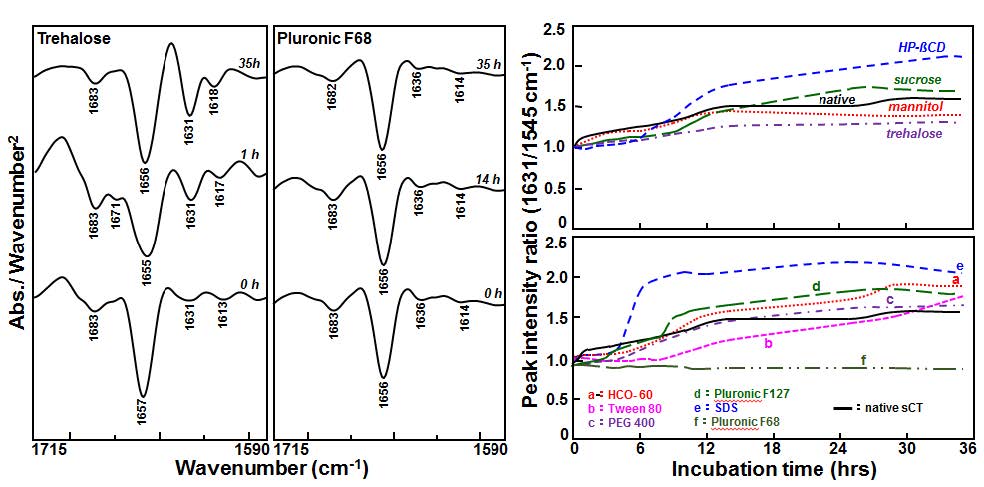
[118]	Lee TH, Lin SY (2011) Pluronic F68 enhanced the conformational stability of salmon calcitonin in both aqueous solution and lyophilized solid form. Biopolymers 95: 785-791.
[119]	Lee TH, Lin SY (2011) Additives affecting thermal stability of salmon calcitonin in aqueous solution and structural similarity in lyophilized solid form. Process Biochem 46: 2163-2169. doi: 10.1016/j.procbio.2011.08.017
[120]	Andreotti G, Méndez BL, Amodeo P, et al. (2006) Structural determinants of salmon calcitonin bioactivity: the role of the Leu-based amphipathic alpha-helix. J Biol Chem 281: 24193-24203. doi: 10.1074/jbc.M603528200
[121]	Carpenter JF, Prestrelski SJ, Dong A (1998) Application of infrared spectroscopy to development of stable lyophilized protein formulations. Eur J Pharm Biopharm 45: 231-238. doi: 10.1016/S0939-6411(98)00005-8
[122]	Haris PI, Chapman D (1994) Analysis of polypeptide and protein structures using Fourier transform infrared spectroscopy. Methods Mol Biol 22: 183-202.
[123]	Pedone E, Bartolucci S, Rossi M, et al. (2003) Structural and thermal stability analysis of Escherichia coli and Alicyclobacillus acidocaldarius thioredoxin revealed a molten globule-like state in thermal denaturation pathway of the proteins: an infrared spectroscopic study. Biochem J 373: 875-883. doi: 10.1042/bj20021747
[124]	Cook TJ, Shenoy SS (2002) Stability of calcitonin salmon in nasal spray at elevated temperatures. Am J Health Syst Pharm 59: 713-715.
[125]	Lee KC, Lee YJ, Song HM, et al. (1992) Degradation of synthetic salmon calcitonin in aqueous solution. Pharm Res 9: 1521-1523. doi: 10.1023/A:1015839719618
[126]	Windisch V, DeLuccia F, Duhau L, et al. (1997) Degradation pathways of salmon calcitonin in aqueous solution. J Pharm Sci 86: 359-364. doi: 10.1021/js9602305
[127]	Kamihira M, Naito A, Tuzi S, et al. (2000) Conformational transitions and fibrillation mechanism of human calcitonin as studied by high-resolution solid-state ¹³C NMR. Protein Sci 9: 867-877. doi: 10.1110/ps.9.5.867
[128]	Andreotti G, Motta A (2004) Modulating calcitonin fibrillogenesis: an antiparallel alpha-helical dimer inhibits fibrillation of salmon calcitonin. J Biol Chem 279: 6364-6370.
[129]	Gaudiano MC, Colone M, Bombelli C, et al. (2005) Early stages of salmon calcitonin aggregation: effect induced by ageing and oxidation processes in water and in the presence of model membranes. Biochim Biophys Acta 1750: 134-145. doi: 10.1016/j.bbapap.2005.04.008
[130]	Diociaiuti M, Macchia G, Paradisi S, et al. (2014) Native metastable prefibrillar oligomers are the most neurotoxic species among amyloid aggregates. Biochim Biophys Acta 1842: 1622-1629. doi: 10.1016/j.bbadis.2014.06.006
[131]	Gilchrist PJ, Bradshow JP (1993) Amyloid formation by salmon calcitonin. Biochim Biophys Acta 1182: 111-114. doi: 10.1016/0925-4439(93)90160-3
[132]	Arvinte T, Cudd A, Drake AF (1993) The structure and mechanism of formation of human calcitonin fibrils. J Biol Chem 268: 6415-6422.
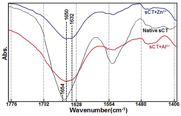
[133]	Rastogi N, Mitra K, Kumar D, et al. (2012) Metal ions as cofactors for aggregation of therapeutic peptide salmon calcitonin. Inorg Chem 51: 5642-5650. doi: 10.1021/ic202604v
[134]	Diociaiuti M, Macchia G, Paradisi S, et al. (2014) Native metastable prefibrillar oligomers are the most neurotoxic species among amyloid aggregates. Biochim Biophys Acta 1842: 1622-1629. doi: 10.1016/j.bbadis.2014.06.006
[135]	Rawat A, Kumar D (2013) NMR investigations of structural and dynamics features of natively unstructured drug peptide-salmon calcitonin: implication to rational design of potent sCT analogs. J Pept Sci 19: 33-45. doi: 10.1002/psc.2471
[136]	Allison SD, Randolph TW, Manning MC, et al. (1998) Effects of drying methods and additives on structure and function of actin: mechanisms of dehydration-induced damage and its inhibition. Arch Biochem Biophys 358: 171-181. doi: 10.1006/abbi.1998.0832
[137]	Bhatnagar BS, Bogner RH, Pikal MJ (2007) Protein stability during freezing: separation of stresses and mechanisms of protein stabilization. Pharm Dev Technol 12: 505-523.
[138]	Jain NK, Roy I (2009) Effect of trehalose on protein structure. Protein Sci 18: 24-36.
[139]	Capelle MA, Gurny R, Arvinte T (2007) High throughput screening of protein formulation stability: practical considerations. Eur J Pharm Biopharm 65: 131-148. doi: 10.1016/j.ejpb.2006.09.009
[140]	Kamerzell TJ, Esfandiary R, Joshi SB, et al. (2011) Protein-excipient interactions: mechanisms and biophysical characterization applied to protein formulation development. Adv Drug Deliv Rev 63: 1118-1159. doi: 10.1016/j.addr.2011.07.006
[141]	Ohtake S, Kita Y, Arakawa T (2011) Interactions of formulation excipients with proteins in solution and in the dried state. Adv Drug Deliv Rev 63: 1053-1073. doi: 10.1016/j.addr.2011.06.011
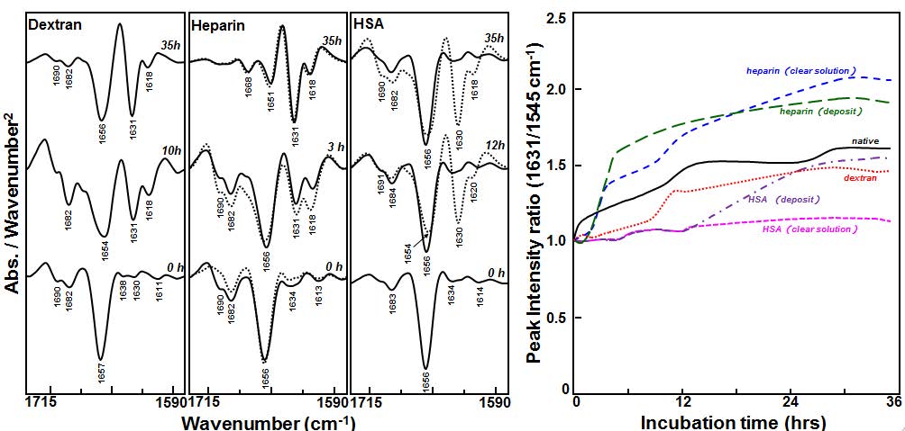
[142]	Porfire AS, Tomuţa I, Irache JM, et al. (2009) The influence of the formulation factors on physico-chemical properties of dextran associated Gantrez an nanoparticles. Farmacia 57: 463-472.
[143]	Torres-Lugo M, Peppas NA (1999) Molecular design and in vitro studies of novel pH-sensitive hydrogels for the oral delivery of calcitonin. Macromolecules 32: 6646-6651.
[144]	Szelke H, Schübel S, Harenberg J, et al. (2010) Interaction of heparin with cationic molecular probes: probe charge is a major determinant of binding stoichiometry and affinity. Bioorg Med Chem Lett 20: 1445-1447. doi: 10.1016/j.bmcl.2009.12.105
[145]	Houska M, Brynda E (1997) Interactions of proteins with polyelectrolytes at solid/liquid interfaces: Sequential adsorption of albumin and heparin. J Colloid Interface Sci 188: 243-250. doi: 10.1006/jcis.1996.4576
[146]	Guo B, Anzai J, Osa T (1996) Adsorption behavior of serum albumin on electrode surfaces and the effects of electrode potential. Chem Pharm Bull (Tokyo) 44: 800-803. doi: 10.1248/cpb.44.800
[147]	Langer K, Balthasar S, Vogel V, et al. (2003) Optimization of the preparation process for human serum albumin (HSA) nanoparticles. Int J Pharm 257: 169-180. doi: 10.1016/S0378-5173(03)00134-0
[148]	Prestrelski SJ, Pikal KA, Arakawa T (1995) Optimization of lyophilization conditions for recombinant human interleukin-2 by dried-state conformational analysis using fourier-transform infrared spectroscopy. Pharm Res 12: 1250-1259. doi: 10.1023/A:1016296801447
[149]	van Dijkhuizen-Radersma R, Nicolas HM, van de Weert M, et al. (2002) Stability aspects of salmon calcitonin entrapped in poly(ether-ester) sustained release systems. Int J Pharm 248: 229-237. doi: 10.1016/S0378-5173(02)00458-1
[150]	Baudys M, Mix D, Kim SW (1996) Stabilization and intestinal absorption of human calcitonin. J Control Rel 39: 145-151. doi: 10.1016/0168-3659(95)00148-4
[151]	Sigurjónsdóttir JF, Loftsson T, Másson M (1999) Influence of cyclodextrins on the stability of the peptide salmon calcitonin in aqueous solution. Int J Pharm 186: 205-213. doi: 10.1016/S0378-5173(99)00183-0
[152]	Mueller C, Capelle MA, Arvinte T, et al. (2011) Noncovalent pegylation by dansyl-poly(ethylene glycol)s as a new means against aggregation of salmon calcitonin. J Pharm Sci 100: 1648-1662. doi: 10.1002/jps.22401
[153]	Mueller C, Capelle MA, Arvinte T, et al. (2011) Tryptophan-mPEGs: novel excipients that stabilize salmon calcitonin against aggregation by non-covalent PEGylation. Eur J Pharm Biopharm 79: 646-657. doi: 10.1016/j.ejpb.2011.06.003
[154]	Mueller C, Capelle MA, Seyrek E, et al. (2012) Noncovalent PEGylation: different effects of dansyl-, L-tryptophan-, phenylbutylamino-, benzyl- and cholesteryl-PEGs on the aggregation of salmon calcitonin and lysozyme. J Pharm Sci 101: 1995-2008. doi: 10.1002/jps.23110
[155]	Remmele RL, Krishnan S, Callahan WJ (2012) Development of stable lyophilized protein drug products. Curr Pharm Biotechnol 13: 471-496. doi: 10.2174/138920112799361990
[156]	Kasper JC, Friess W (2011) The freezing step in lyophilization: physico-chemical fundamentals, freezing methods and consequences on process performance and quality attributes of biopharmaceuticals. Eur J Pharm Biopharm 78: 248-263. doi: 10.1016/j.ejpb.2011.03.010
[157]	Costantino HR, Pikal MJ (2004) Lyophilization of Biopharmaceuticals. Virginia: AAPS Press.
[158]	Susi H, Byler DM (1983) Protein structure by Fourier transform infrared spectroscopy: second derivative spectra. Biochem Biophys Res Commun 115: 391-397. doi: 10.1016/0006-291X(83)91016-1
[159]	Prestrelski SJ, Tedeschi N, Arakawa T, et al. (1993) Dehydration-induced conformational transitions in proteins and their inhibition by stabilizers. Biophys J 65: 661-671. doi: 10.1016/S0006-3495(93)81120-2
[160]	Lee HE, Lee MJ, Park CR, et al. (2010) Preparation and characterization of salmon calcitonin-sodium triphosphate ionic complex for oral delivery. J Control Rel 143: 251-257. doi: 10.1016/j.jconrel.2009.12.011
[161]	Steckel H, Brandes HG (2004) A novel spray-drying technique to produce low density particles for pulmonary delivery. Int J Pharm 278: 187-195. doi: 10.1016/j.ijpharm.2004.03.010
[162]	Seville PC, Li HY, Learoyd TP (2007) Spray-dried powders for pulmonary drug delivery. Crit Rev Ther Drug Carrier Syst 24: 307-360. doi: 10.1615/CritRevTherDrugCarrierSyst.v24.i4.10
[163]	Sollohub K, Cal K (2010) Spray drying technique: II. Current applications in pharmaceutical technology. J Pharm Sci 99: 587-597.
[164]	Telko M, Hickey A (2005) Dry powder inhaler formulation. Respir Care 50: 1209-1227.
[165]	Ameri M, Maa Y (2006) Spray Drying of Biopharmaceuticals: Stability and Process Considerations. Drying Technol: A Int J 24: 763-768. doi: 10.1080/03602550600685275
[166]	Chan HK, Clark AR, Feeley JC, et al. (2004) Physical stability of salmon calcitonin spray-dried powders for inhalation. J Pharm Sci 93: 792-804. doi: 10.1002/jps.10594
[167]	Yang M, Velaga S, Yamamoto H, et al. (2007) Characterisation of salmon calcitonin in spray-dried powder for inhalation. Effect of chitosan. Int J Pharm 331: 176-181.
[168]	Sinsuebpol C, Chatchawalsaisin J, Kulvanich P (2013) Preparation and in vivo absorption evaluation of spray dried powders containing salmon calcitonin loaded chitosan nanoparticles for pulmonary delivery. Drug Des Devel Ther 7: 861-873.
[169]	Amaro MI, Tewes F, Gobbo O, et al. (2015) Formulation, stability and pharmacokinetics of sugar-based salmon calcitonin-loaded nanoporous/nanoparticulate microparticles (NPMPs) for inhalation. Int J Pharm 483: 6-18.
[170]	Lechuga-Ballesteros D, Charan C, Stults CL, et al. (2008) Trileucine improves aerosol performance and stability of spray-dried powders for inhalation. J Pharm Sci 97: 287-302. doi: 10.1002/jps.21078
[171]	Tewes F, Gobbo OL, Amaro MI, et al. (2011) Evaluation of HP βCD-PEG microparticles for salmon calcitonin administration via pulmonary delivery. Mol Pharm 8: 1887-1898. doi: 10.1021/mp200231c
[172]	Epand RM, Epand RF, Orlowski RC, et al. (1983) Amphipathic helix and its relationship to the interaction of calcitonin with phospholipids. Biochemistry 22: 5074-5084.
[173]	Epand RM, Epand RF (1986) Conformational flexibility and biological activity of salmon calcitonin. Biochemistry 25: 1964-1968.
[174]	Green FR 3rd, Lynch B, Kaiser ET (1987) Biological and physical properties of a model calcitonin containing a glutamate residue interrupting the hydrophobic face of the idealized amphiphilic alpha-helical region. Proc Natl Acad Sci U S A 84: 8340-8344. doi: 10.1073/pnas.84.23.8340
[175]	Nabuchi Y, Asoh Y, Takayama M (2004) Folding analysis of hormonal polypeptide calcitonins and the oxidized calcitonins using electrospray ionization mass spectrometry combined with H/D exchange. J Am Soc Mass Spectrom 15: 1556-1564. doi: 10.1016/j.jasms.2004.07.007
[176]	Siligardi G, Samorí B, Melandri S, et al. (1994) Correlations between biological activities and conformational properties for human, salmon, eel, porcine calcitonins and Elcatonin elucidated by CD spectroscopy. Eur J Biochem 221: 1117-1125. doi: 10.1111/j.1432-1033.1994.tb18832.x
[177]	Andreotti G, Méndez BL, Amodeo P, et al. (2006) Structural determinants of salmon calcitonin bioactivity: the role of the Leu-based amphipathic alpha-helix. J Biol Chem 281: 24193-24203. doi: 10.1074/jbc.M603528200
[178]	Stefani M (2004) Protein misfolding and aggregation: new examples in medicine and biology of the dark side of the protein world. Biochim Biophys Acta 1739: 5-25. doi: 10.1016/j.bbadis.2004.08.004
[179]	Renukuntla J, Vadlapudi AD, Patel A, et al. (2013) Approaches for enhancing oral bioavailability of peptides and proteins. Int J Pharm 447: 75-93. doi: 10.1016/j.ijpharm.2013.02.030
[180]	Choonara BF, Choonara YE, Kumar P, et al. (2014) A review of advanced oral drug delivery technologies facilitating the protection and absorption of protein and peptide molecules. Biotechnol Adv 32: 1269-1282. doi: 10.1016/j.biotechadv.2014.07.006
[181]	Smart AL, Gaisford S, Basit AW (2014) Oral peptide and protein delivery: intestinal obstacles and commercial prospects. Expert Opin Drug Deliv 11: 1323-1335. doi: 10.1517/17425247.2014.917077
[182]	Franks F, Hatley RHM, Mathias SF (1991) Materials science and the production of shelf-stable biologicals. Pharm Technol Int 3: 24-34.
[183]	Slade L, Levine H (1991) Beyond water activity: Recent advances based on an alternative approach to the assessment of food quality and safety. Crit Rev Food Sci Nutri 30: 115-360. doi: 10.1080/10408399109527543
[184]	Carpenter JF, Prestrelski SJ, Arakawa T (1993) Separation of freezing- and drying-induced denaturation of lyophilized proteins using stress-specific stabilization. I. Enzyme activity and calorimetric studies. Arch Biochem Biophys 303: 456-464.
[185]	Carpenter JF, Crowe JH (1989) An infrared spectroscopic study of the interactions of carbohydrates with dried proteins. Biochemistry 28: 3916-3922. doi: 10.1021/bi00435a044
[186]	Crowe JH, Crowe LM, Carpenter JF (1993) Preserving dry biomaterials: The water replacement hypothesis, Part 1. BioPharm 6: 28-29, 32-33.
[187]	Crowe JH, Crowe LM, Carpenter JF (1993) Preserving dry biomaterials: the water replacement hypothesis, Part 2. BioPharm 6: 40-43.

This article has been cited by:

1.	Ajay Singh Rathore, Vembu Shanthi, A numerical solution of singularly perturbed Fredholm integro-differential equation with discontinuous source term, 2024, 446, 03770427, 115858, 10.1016/j.cam.2024.115858
2.	Abhilipsa Panda, Jugal Mohapatra, Ilhame Amirali, Muhammet Enes Durmaz, Gabil M. Amiraliyev, A numerical technique for solving nonlinear singularly perturbed Fredholm integro-differential equations, 2024, 220, 03784754, 618, 10.1016/j.matcom.2024.02.011

Reader Comments

Your name:*

Email:*
© 2015 the Author(s), licensee AIMS Press. This is an open access article distributed under the terms of the Creative Commons Attribution License (http://creativecommons.org/licenses/by/4.0)