Experiments with pedestrians revealed that the geometry of the domain, as well as the incentive of pedestrians to reach a target as fast as possible have a strong influence on the overall dynamics. In this paper, we propose and validate different mathematical models at the micro- and macroscopic levels to study the influence of both effects. We calibrate the models with experimental data and compare the results at the micro- as well as macroscopic levels. Our numerical simulations reproduce qualitative experimental features on both levels, and indicate how geometry and motivation level influence the observed pedestrian density. Furthermore, we discuss the dynamics of solutions for different modeling approaches and comment on the analysis of the respective equations.
Citation: Michael Fischer, Gaspard Jankowiak, Marie-Therese Wolfram. Micro- and macroscopic modeling of crowding and pushing in corridors[J]. Networks and Heterogeneous Media, 2020, 15(3): 405-426. doi: 10.3934/nhm.2020025
Experiments with pedestrians revealed that the geometry of the domain, as well as the incentive of pedestrians to reach a target as fast as possible have a strong influence on the overall dynamics. In this paper, we propose and validate different mathematical models at the micro- and macroscopic levels to study the influence of both effects. We calibrate the models with experimental data and compare the results at the micro- as well as macroscopic levels. Our numerical simulations reproduce qualitative experimental features on both levels, and indicate how geometry and motivation level influence the observed pedestrian density. Furthermore, we discuss the dynamics of solutions for different modeling approaches and comment on the analysis of the respective equations.

| [1] |
Crowding and queuing at entrances, (2018), http://ped.fz-juelich.de/da/doku.php?id=wuptmp. |
| [2] |
Jupedsim, (2019), https://www.jupedsim.org. |
| [3] |
J. Adrian, M. Boltes, S. Holl, A. Sieben and A. Seyfried, Crowding and queuing in entrance scenarios: Influence of corridor width in front of bottlenecks, arXiv e-prints, arXiv: 1810.07424. |
| [4] |
When push comes to shove: Exclusion processes with nonlocal consequences. Physica A (2015) 437: 119-129. 
|
| [5] |
M. Bardi and I. Capuzzo-Dolcetta, Optimal Control and Viscosity Solutions of Hamilton-Jacobi-Bellman Equations, Systems & Control: Foundations & Applications, Birkhäuser Boston, Inc., Boston, MA, 1997. |
| [6] |
Lane formation by side-stepping. SIAM Journal on Mathematical Analysis (2016) 48: 981-1005.
|
| [7] |
Flow characteristics in a crowded transport model. Nonlinearity (2016) 29: 3528-3550.
|
| [8] |
Simulation of pedestrian dynamics using a two-dimensional cellular automaton. Physica A: Statistical Mechanics and its Applications (2001) 295: 507-525.
|
| [9] |
Distance functions and almost global solutions of eikonal equations. Communications in Partial Differential Equations (2010) 35: 391-414.
|
| [10] |
A. Corbetta, J. A. Meeusen, C.-m. Lee, R. Benzi and F. Toschi, Physics-based modeling and data representation of pairwise interactions among pedestrians, Physical Review E, 98 (2018), 062310. |
| [11] |
E. Cristiani, B. Piccoli and A. Tosin, Multiscale Modeling of Pedestrian Dynamics, MS & A, Modeling, Simulation and Applications, 12. Springer, Cham, 2014. |
| [12] |
On the Hughes' model for pedestrian flow: The one-dimensional case. Journal of Differential Equations (2011) 250: 1334-1362.
|
| [13] |
D. C. Duives, W. Daamen and S. Hoogendoorn, Trajectory analysis of pedestrian crowd movements at a Dutch music festival, Pedestrian and Evacuation Dynamics 2012, Springer, (2014), 151–166. |
| [14] |
Parameter estimation for macroscopic pedestrian dynamics models from microscopic data. SIAM Journal on Applied Mathematics (2019) 79: 1475-1500.
|
| [15] |
B. Hein, Agent-Based Modelling for Crowding and Queuing in Front of Bottlenecks, Bachelor's Thesis, University of Wuppertal, 2019. |
| [16] |
D. Helbing and P. Molnár, Social force model for pedestrian dynamics, Physical Review E, 51 (1995), 4282. |
| [17] |
K. Hirai and K. Tarui, A simulation of the behavior of a crowd in panic, Systems and Control. |
| [18] |
A continuum theory for the flow of pedestrians. Transportation Research Part B: Methodological (2002) 36: 507-535.
|
| [19] |
A. Johansson and D. Helbing, Analysis of empirical trajectory data of pedestrians, Pedestrian and Evacuation Dynamics 2008, (2009), 203–214. |
| [20] |
A. Jüngel, The boundedness-by-entropy method for cross-diffusion systems, Nonlinearity, 28 (2015), 1963. |
| [21] |
Simulation of evacuation processes using a bionics-inspired cellular automaton model for pedestrian dynamics. Physica A: Statistical Mechanics and its Applications (2002) 312: 260-276.
|
| [22] |
C. Koutschan, H. Ranetbauer, G. Regensburger and M.-T. Wolfram, Symbolic derivation of mean-field PDEs from lattice-based models, 2015 17th International Symposium on Symbolic and Numeric Algorithms for Scientific Computing (SYNASC), 27–33. |
| [23] |
O. Ladyzhenskaya, Linear and Quasilinear Elliptic Equations, ISSN, Elsevier Science, 1968. |
| [24] |
Explicit formula for scalar nonlinear conservation laws with boundary condition. Mathematical Methods in the Applied Sciences (1988) 10: 265-287.
|
| [25] |
Explicit formula for weighted scalar nonlinear hyperbolic conservation laws. Transactions of the American Mathematical Society (1988) 308: 667-683.
|
| [26] |
C. Lehrenfeld, On a Space-Time Extended Finite Element Method for the Solution of a Class of Two-Phase Mass Transport Problems, PhD thesis, RWTH Aachen, 2015, http://publications.rwth-aachen.de/record/462743. |
| [27] |
A. Y. Leroux, Approximation de Quelques Problèmes Hyperboliques Non-Linéaires, Thèse d'état, Rennes, 1979. |
| [28] |
B. Maury and S. Faure, Crowds in Equations. An Introduction to the Microscopic Modeling of Crowds, Advanced Textbooks in Mathematics. World Scientific Publishing Co. Pte. Ltd., Hackensack, NJ, 2019. |
| [29] |
Experimental study of the behavioural mechanisms underlying self-organization in human crowds. Proceedings of The Royal Society B: Biological Sciences (2009) 276: 2755-2762.
|
| [30] |
S. Nowak and A. Schadschneider, Quantitative analysis of pedestrian counterflow in a cellular automaton model, Physical Review E, 85 (2012), 066128. |
| [31] |
S. Okazaki, A study of pedestrian movement in architectural space, Trans. of A.I.J., 283. |
| [32] |
Time-evolving measures and macroscopic modeling of pedestrian flow. Archive for Rational Mechanics and Analysis (2011) 199: 707-738.
|
| [33] |
Fast sweeping methods for eikonal equations on triangular meshes. SIAM J. Numerical Analysis (2007) 45: 83-107.
|
| [34] |
C. Rudloff, T. Matyus and S. Seer, Comparison of different calibration techniques on simulated data, Pedestrian and Evacuation Dynamics 2012, Springer, (2013), 657–672. |
| [35] |
A. Schadschneider, C. Eilhardt, S. Nowak and R. Will, Towards a calibration of the floor field cellular automaton, Pedestrian and Evacuation Dynamics, (2011), 557–566. |
| [36] |
A. Schadschneider, H. Klpfel, T. Kretz, C. Rogsch and A. Seyfried, Fundamentals of pedestrian and evacuation dynamics, IGI Global, (2009), 124–154. |
| [37] |
Comparative study of macroscopic pedestrian models. Transportation Research Procedia (2014) 2: 477-485.
|
| [38] |
U. Weidmann, Transporttechnik der Fussgänger: Transporttechnische Eigenschaften des Fussgängerverkehrs, Schriftenreihe des IVT, IVT, 1993. |
| [39] |
W. G. Weng, T. Chen, H. Y. Yuan and W. C. Fan, Cellular automaton simulation of pedestrian counter flow with different walk velocities, Physical Review. E, 74 (2006), 036102. |
| [40] |
C. A. Yates, A. Parker and R. E. Baker, Incorporating pushing in exclusion-process models of cell migration, Physical Review E, 91 (2015), 052711. |
Figures(14) / Tables(1)
Michael Fischer, Gaspard Jankowiak, Marie-Therese Wolfram. Micro- and macroscopic modeling of crowding and pushing in corridors[J]. Networks and Heterogeneous Media, 2020, 15(3): 405-426. doi: 10.3934/nhm.2020025

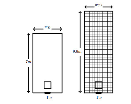
Left: Sketch of experimental setup at the University of Wuppertal, showing the corridor width
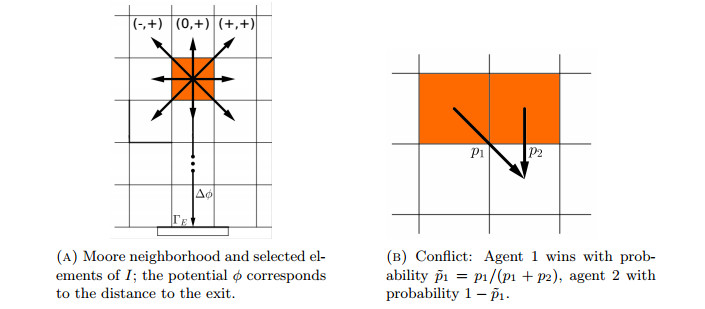
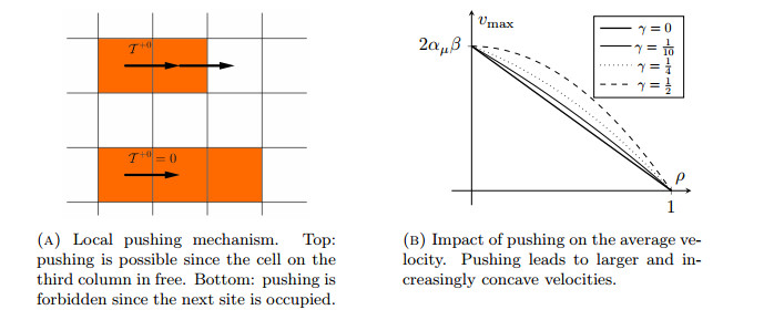
Cellular automaton: transition rules
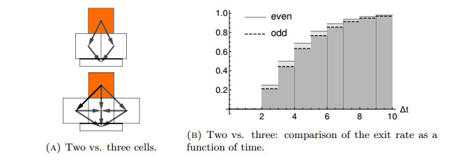
Discretization of the exit. In the case of an even number of cells, a central positioned agent will leave the corridor faster than in the case of three cells
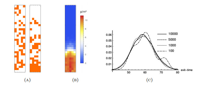
(A) distribution of
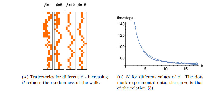
Influence of the scaling parameter
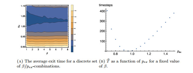
Average exit time as a function of
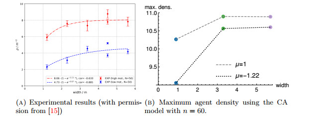
Impact of the corridor width on the maximum density. The CA approach yields comparable results for high density regimes and low motivation level
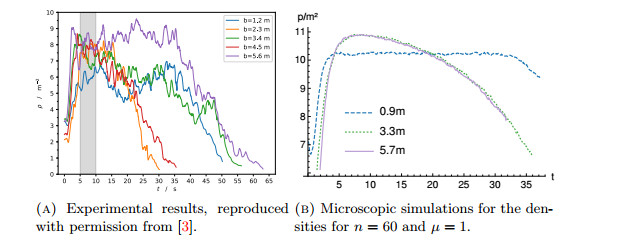
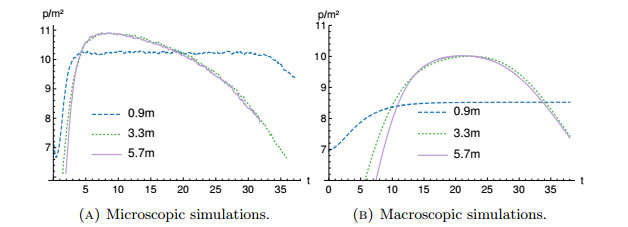
Impact of the motivation level on the maximum pedestrian density: experimental (A) vs. microscopic simulations (B)
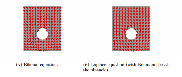
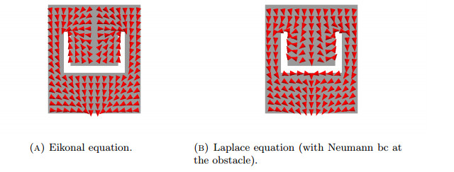
Comparison of the potentials
Comparison of the potentials
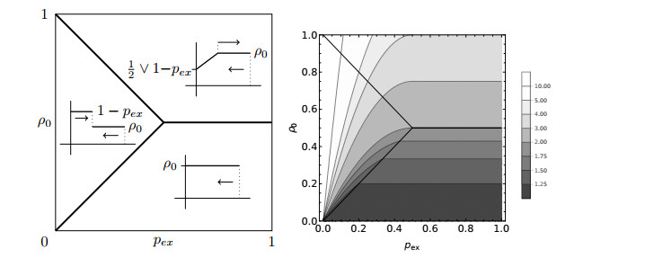
Left: Bifurcation diagram detailing the behavior of the solution to (12)-(13). The behavior along the interface lines is identical as in the bottom right corner. Right: exit time corresponding to
Simulations for
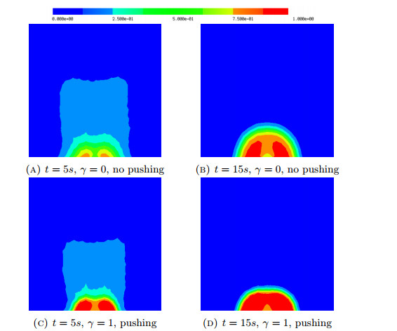
Effects of pushing
Comparison of the congestion at the exit in case of pushing (bottom row) and no-pushing (top row) for


 DownLoad: