
A directed graph
The methodology named LIFE (Linear-in-Flux-Expressions) was developed with the purpose of simulating and analyzing large metabolic systems. With LIFE, the number of model parameters is reduced by accounting for correlations among the parameters of the system. Perturbation analysis on LIFE systems results in less overall variability of the system, leading to results that more closely resemble empirical data. These systems can be associated to graphs, and characteristics of the graph give insight into the dynamics of the system.
This work addresses two main problems: 1. for fixed metabolite levels, find all fluxes for which the metabolite levels are an equilibrium, and 2. for fixed fluxes, find all metabolite levels which are equilibria for the system. We characterize the set of solutions for both problems, and show general results relating stability of systems to the structure of the associated graph. We show that there is a structure of the graph necessary for stable dynamics. Along with these general results, we show how stability analysis from the fields of network flows, compartmental systems, control theory and Markov chains apply to LIFE systems.
Citation: Nathaniel J. Merrill, Zheming An, Sean T. McQuade, Federica Garin, Karim Azer, Ruth E. Abrams, Benedetto Piccoli. Stability of metabolic networks via Linear-in-Flux-Expressions[J]. Networks and Heterogeneous Media, 2019, 14(1): 101-130. doi: 10.3934/nhm.2019006
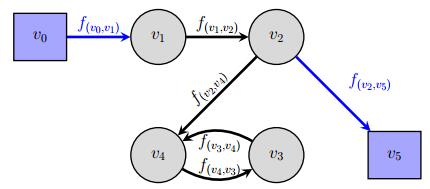
[1] | Nathaniel J. Merrill, Zheming An, Sean T. McQuade, Federica Garin, Karim Azer, Ruth E. Abrams, Benedetto Piccoli . Stability of metabolic networks via Linear-in-Flux-Expressions. Networks and Heterogeneous Media, 2019, 14(1): 101-130. doi: 10.3934/nhm.2019006 |
[2] | Maya Briani, Emiliano Cristiani . An easy-to-use algorithm for simulating traffic flow on networks: Theoretical study. Networks and Heterogeneous Media, 2014, 9(3): 519-552. doi: 10.3934/nhm.2014.9.519 |
[3] | Gildas Besançon, Didier Georges, Zohra Benayache . Towards nonlinear delay-based control for convection-like distributed systems: The example of water flow control in open channel systems. Networks and Heterogeneous Media, 2009, 4(2): 211-221. doi: 10.3934/nhm.2009.4.211 |
[4] | Thibault Liard, Raphael Stern, Maria Laura Delle Monache . A PDE-ODE model for traffic control with autonomous vehicles. Networks and Heterogeneous Media, 2023, 18(3): 1190-1206. doi: 10.3934/nhm.2023051 |
[5] | Edward S. Canepa, Alexandre M. Bayen, Christian G. Claudel . Spoofing cyber attack detection in probe-based traffic monitoring systems using mixed integer linear programming. Networks and Heterogeneous Media, 2013, 8(3): 783-802. doi: 10.3934/nhm.2013.8.783 |
[6] | Mahmoud Saleh, Endre Kovács, Nagaraja Kallur . Adaptive step size controllers based on Runge-Kutta and linear-neighbor methods for solving the non-stationary heat conduction equation. Networks and Heterogeneous Media, 2023, 18(3): 1059-1082. doi: 10.3934/nhm.2023046 |
[7] | Paola Goatin, Chiara Daini, Maria Laura Delle Monache, Antonella Ferrara . Interacting moving bottlenecks in traffic flow. Networks and Heterogeneous Media, 2023, 18(2): 930-945. doi: 10.3934/nhm.2023040 |
[8] | Ginestra Bianconi, Riccardo Zecchina . Viable flux distribution in metabolic networks. Networks and Heterogeneous Media, 2008, 3(2): 361-369. doi: 10.3934/nhm.2008.3.361 |
[9] | Riccardo Bonetto, Hildeberto Jardón Kojakhmetov . Nonlinear diffusion on networks: Perturbations and consensus dynamics. Networks and Heterogeneous Media, 2024, 19(3): 1344-1380. doi: 10.3934/nhm.2024058 |
[10] | Didier Georges . Infinite-dimensional nonlinear predictive control design for open-channel hydraulic systems. Networks and Heterogeneous Media, 2009, 4(2): 267-285. doi: 10.3934/nhm.2009.4.267 |
The methodology named LIFE (Linear-in-Flux-Expressions) was developed with the purpose of simulating and analyzing large metabolic systems. With LIFE, the number of model parameters is reduced by accounting for correlations among the parameters of the system. Perturbation analysis on LIFE systems results in less overall variability of the system, leading to results that more closely resemble empirical data. These systems can be associated to graphs, and characteristics of the graph give insight into the dynamics of the system.
This work addresses two main problems: 1. for fixed metabolite levels, find all fluxes for which the metabolite levels are an equilibrium, and 2. for fixed fluxes, find all metabolite levels which are equilibria for the system. We characterize the set of solutions for both problems, and show general results relating stability of systems to the structure of the associated graph. We show that there is a structure of the graph necessary for stable dynamics. Along with these general results, we show how stability analysis from the fields of network flows, compartmental systems, control theory and Markov chains apply to LIFE systems.
Quantitative Systems Pharmacology (QSP) aims to gain more information about a potential drug treatment on a human patient before the more expensive stages of development begin [22]. QSP models allow us to perform in silico experiments on a simulated metabolic system that predicts the response of perturbing a flux. A drug may be metabolized differently by various patients, and modelers working in pharmacology must anticipate these differences. Building a profile of how the drug affects different classes of simulated patients will help the developers of new drugs understand the viability of a treatment and acquire insight into the mechanisms by which the drug acts.
A recent advancement in QSP modeling called Linear-in-Flux-Expressions (LIFE) is a method of analyzing systems of Ordinary Differential Equations (ODEs) [19,18]. Originally, LIFE was designed to analyze metabolic systems, which are composed of Fluxes and Metabolites. Fluxes in the metabolic system are the rates of chemical reactions in the human body, and they determine the dynamics on the metabolites, which are the various chemical compounds involved in metabolism. Modeling these systems depends on choosing fluxes, which are difficult to measure directly, so that the system effectively simulates human metabolism.
To implement LIFE on a metabolic network, the network must be written as a directed graph [18]. The edges of the graph represent the reaction rates (fluxes), and the vertices represent quantities of chemical compounds (metabolites). From the graph we construct the stoichiometric matrix of the system. This stoichiometric matrix is not the classical one mentioned by [21,24]. The LIFE method is also different from QSP models whose dynamics traditionally depend on a matrix containing information about the flux of the system. In these classical QSP models the dynamics of the metabolites are linear with respect to the metabolites. By contrast, systems using the LIFE method are linear in fluxes and have a stoichiometric matrix that is dependent on the metabolites.
Initially, the LIFE method was developed using the human cholesterol metabolism network [19]. LIFE enables us to simply describe the correlations among the fluxes of the model at steady state. There are generally many correlations among fluxes, and maintaining these correlations leads to a more consistent response to perturbing the fluxes in the system. This was advantageous to QSP modelers, who previously analyzed flux perturbations with little to no consideration to relationships among fluxes [1]. Now, we expand our study of these systems, showing that with few assumptions, systems that are linear in the flux is stable.
The LIFE method evolved from methods in systems biology [21]. Systems biology, in conjunction with network flows [12,9], Markov chains [6], laplacian dynamics [13], control theory [3], and compartmental systems [4,14] allow us to better understand biological networks on which pharmacology models are based. The field of compartmental systems focuses on models based on directed graphs. Vertices of the graph represent quantities whose dynamics are determined by the edges of the graph, which represent fluxes among compartments. Markov chains study dynamics on directed graphs as well, but by contrast, this field focuses on stochastic processes. Control theory studies the way an external agent can alter the natural evolution of a system, given a set of admissible controls. In pharmacology, metabolism follows its natural evolution, and drugs serve as our controls. These fields have much to contribute to systems pharmacology, and we summarize useful results. We identify assumptions which are usually satisfied by real metabolic networks, guaranteeing stability of the metabolic system at a unique equilibrium.
The paper is organized as follows. In section 2, we describe the model system for the LIFE approach in the form of a system of ODEs associated to a metabolic networks, then show existence of positive solutions and provide results of equilibria under general assumptions. Also special classes of LIFE systems are introduced. Section 3 investigates the flow vectors for which a given metabolite vector
We indicate by
We introduce some terminology commonly used in graph theory. A directed graph is a couple
A terminal component of a directed graph
We indicate by
$ dxdt=F(x,f), $
|
(1) |
$ dfdt=G(x,f), $
|
(2) |
where
The dynamics (1) is very general and we restrict to special system, which are linear in the fluxes, thus can be written as:
$ ˙x=S(x)⋅f $
|
(3) |
where
We now illustrate how to construct a directed graph from the metabolic network for the system (3). We represent metabolites with vertices
Example 2.1. To illustrate the concepts of graph with virtual vertices and stoichiometric matrix related to a metabolic network, we provide a toy example with linear dynamics. Consider the system given by the following stoichiometric matrix and fluxes vector:
$ S(x)=(1−x1−x1000x40x10−x200000x1x2−x3−x300000x30−x4),f=(f(v0,v1)f(v1,v2)f(v1,v3)f(v2,v3)f(v3,v4)f(v3,v5)f(v4,v1)). $
|
Then the corresponding graph is represented in Figure 2.
Remark 1. It is worth a reminder that our stoichiometric matrix is different from the traditional one defined by [21,24], in which entries are stoichiometric coefficients, i.e. do not depend on metabolites.
To correctly represent the reactions corresponding to fluxes (which take always strictly positive values), we assume:
(A) For
$ Sve(x)={He(x)>0if e=(w,v), w∈V and xv>0 or e=(v0,v), v∈I−He(x)<0if e=(v,w), w∈V and xv>0 or e=(v,vn+1), v∈X and xv>00otherwise, $
|
where
Notice that Assumption (A) implies that, for each
$ ∑v∈VSve(x)={He(x)e=(v0,ˉv), ˉv∈I,−He(x)e=(ˉv,vn+1), ˉv∈X,0otherwise, $
|
(4) |
namely all columns of
$ ˙xv=∑e∈˜ESve(x)fe=∑w:(w,v)∈˜EH(w,v)(x)f(w,v)−∑w:(v,w)∈˜EH(v,w)(x)f(v,w), $
|
(5) |
which is the mass balance for metabolite
The total mass in the system is
$ \dot m = \sum\limits_{v \in I} H_{(v_0, v)}(x) f_{(v_0, v)} -\sum\limits_{v \in X} H_{(v, v_{n+1})}(x) f_{(v, v_{n+1})} \, . $ |
Clearly, in the case without intakes nor excretions,
Another remark which is useful is that, under Assumption (A),
In the remainder of this section we study the dynamics (3) under the very general Assumption (A), while later in the paper we add other assumptions, restricting our attention to systems for which stronger statements can be obtained. A first important general property is that positivity of solution is guaranteed:
Proposition 1. Consider a system (3) satisfying (A) and the Cauchy problem with initial datum
Proof. Existence follows from Lipschitz condition, while positivity of solution follows from the invariance of the set
In the next Proposition we show that existence of nontrivial equilibria implies some structure on the network: every vertex
Proposition 2. Consider a system (3) satisfying (A). Assume there exists an equilibrium
Proof. Assume there exists an equilibrium
It is easy to show that
Finally we have a terminal component
The system associated to the graph in Figure 2 provides an explicit example of the contradiction argument of Proposition 2. The vertices
The same system of Figure 2 shows the necessity of the assumption that
Another example not satisfying the assumptions of Proposition 2 is shown in Figure 3. This system admits an equilibrium under Assumption (A) even though the vertex
For general systems (3) with Assumption (A) it is not possible to prove other general conclusions about equilibria, beside Propositions 1 and 2. Indeed consider the simple metabolic network given in Figure 4. Under Assumption (A), the dynamics is written as:
$ {˙xv1=−f(v1,v2)⋅H(v1,v2)(x)+f(vn,v1)⋅H(vn,v1)(x)˙xv2=−f(v2,v3)⋅H(v2,v3)(x)+f(v1,v2)⋅H(v1,v2)(x)˙xv3=−f(v3,v4)⋅H(v3,v4)(x)+f(v2,v3)⋅H(v2,v3)(x)⋮˙xvn=−f(vn,v1)⋅H(vn,v1)(x)+f(vn−1,vn)⋅H(vn−1,vn)(x). $
|
(6) |
We want to show that for any dynamical system in
$ {˙xv1=F1(xv1,xv2,…,xvn)˙xv2=F2(xv1,xv2,…,xvn)⋮˙xvn=Fn(xv1,xv2,…,xvn). $
|
(7) |
we look for a choice of the functions
$ ˙xvn=−˙xv1−⋯−˙xvn−1=n−1∑i=1−Fi. $
|
(8) |
Define the set
Proposition 3. Consider system (7) and assume
Proof. Assign the functions
$ H(vi,vi+1)(x)=∑k≤i[Fk]−+∑ℓ>i[Fℓ]+if i<n,H(vn,v1)(x)=n∑k=1[Fk]+, $
|
(9) |
where
Here we introduce a special class of systems of type (3) with simplified dynamics. We consider Assumption (A), and we impose further restriction on the functions
(B) It holds
$ Sve(x)={−He(xv)e=(v,w), v∈V,w∈V∪{vn+1}He(xw)e=(w,v), w∈V1e=(v0,v) v∈I0otherwise, $
|
(10) |
and each
A typical example of a system verifying (B) is given by metabolic networks with Hill functions representing reactions, i.e.
A further simplification occurs in the case where
(C) It holds
$ Sve(x)={−Hv(xv)e=(v,w), v∈V,w∈V∪{vn+1}Hw(xw)e=(w,v), w∈V1e=(v0,v) v∈I0otherwise, $
|
and each
Under Assumption (C), the system
$ ˙x=J(f)h(x)+ϕ, $
|
(11) |
where
$ J_{ij}(f) = {f(vj,vi)if (vj,vi)∈E−∑w:(vi,w)∈˜Ef(vi,w)ifj=i0otherwise, $
|
where
Finally, the simplest class of LIFE models we consider are linear systems, namely systems satisfying Assumption (C), where each
Example 2.1 (continued). This example is a linear LIFE system. We can equivalently re-write its dynamics
$ J(f) = \left( −f(v1,v2)−f(v1,v3)00f(v4,v1)f(v1,v2)−f(v2,v3)00f(v1,v3)f(v2,v3)−f(v3,v4)−f(v3,v5)000f(v3,v4)−f(v4,v1) \right), \; \phi = \left(f(v0,v1)000 \right). $
|
In this section we consider equilibrium solutions of the system (3) satisfying Assumption (A). In general one is interested in conditions guaranteeing existence of an equilibrium and also in conditions necessary for uniqueness and stability of such an equilibrium. There are two problems: for fixed metabolite concentrations
The set of flux vectors for which
We extend one of the results of [18] to get:
Proposition 4. Consider the system (3) with no intakes nor excretions satisfying Assumption (A) and let
$ {\rm rank}(S(x)) = n-\ell, $ |
where
Proof. We have
Next we consider systems that contain both intakes and excretions. It was shown in [18] that if intakes and excretions are added to a graph satisfying the conditions of Proposition 4 then
Proposition 5. Consider the system (3) satisfying Assumption (A) and let
Proof. It was shown in [18] that if
$ S(x) = (S1(x)0⋱0Sℓ(x)) $
|
where each diagonal element
Notice that the rank of
The problem of finding positive flows admitting an equilibrium with strictly positive entries has been extensively studied in the operations research literature under the name of 'network flow' problems [12]. In network flow problems one considers a directed graph where edges represent flows between the vertices. The maximum flow which an edge can support is called the capacity of the edge. In addition to capacity each edge may also have a cost associated to it. Network flow problems assume that the system is at equilibrium with respect to the vertices i.e. that the flow entering and leaving a vertex must be the same. A flow that satisfies this assumption is called a feasible flow. Finding feasible flows is the same as finding flows in the cone
A flow is a mapping from
Proposition 6 (Max-Flow Min-Cut Theorem). The maximum flow value obtainable in a network is the minimum capacity of all cut sets which disconnect
An implication of the max-flow min-cut theorem is that a feasible flow exists if there is a path from
Proposition 7. Given a LIFE system with graph
Proof. Consider the maximum flow problem on the graph
If for some
There are many standard methods for computing a basis of the nullspace of a matrix [20], and hence to describe
Finding a positive basis for a cone is not as easy as finding a traditional basis. In [21], Palsson describes a method to find a positive basis by using extreme pathways of a metabolic network. The extreme pathways are a unique set of positively independent flux vectors that represent the edges of the cone
Here we summarize a method to build extreme pathways described by [23]. We start considering the equation
Algorithm 1. The algorithm consists of the following steps:
Step 1. Select from
Step 2. Add to
Step 3. Define
Step 4. Remove positively linearly dependent rows from
Step 5. Repeat the steps 1-4 now considering first excretion vertices and then intake vertices until all columns are
If the algorithm stops at step
Originally in [21] the extreme pathways method was proposed for stoichiometric matrices not dependent on
To illustrate the process we report an example using the Reverse Cholesterol Transport Network (RCT) from [19]. The RCT network is shown in Figure 5.
Reverse Cholesterol Transport Network from [19]. This network contains 6 vertices which represent metabolites, 10 edges which represent fluxes and 2 virtual vertices
Example 3.1. Finding Extreme Pathways of RCT network
We use Palsson's algorithm for finding extreme pathways on the stoichiometric matrix from the RCT network. The stoichiometric matrix for RCT is given by:
$ S(x)=(100−x10000000100−x20000000100−x30000000x1x2x3−x4−x400000000x40−x500000000x4x5−x6) $
|
For space, the complete calculations are continued in the Appendix.
Let us first recall Farkas' Lemma [10]. Here we use the notation
Lemma 3.1 (Farkas' Lemma). Let
1. There exists
2. There exists
Proposition 8. The extreme pathways of
Proof. There are three statements which must be shown to prove this Proposition.
Statement 1: The extreme pathway vectors (
Statement 2: The span of the extreme pathways vectors is contained in
Statement 3: The extreme pathways vectors span
Statement 1 follows from Step 4 of the algorithm.
Let us now prove Statement 2. Since the vectors corresponding to extreme pathways are positive combinations of rows of matrices with positive entries, then
Finally it remains to prove statement 3, in order to show
For simplicity of notation, we assume
$ ∑μi,j(ci+αi,jcj)=n∑i=1λici. $
|
(12) |
We can split the sum on the right hand side by considering the positive and negative entries separately,
$ ∑μi,j(ci+αi,jcj)=ℓ∑i=1λici+n∑i=ℓ+1λici. $
|
For
$ ℓ∑k=1μk,iαk,i=λi $
|
which gives:
$ ℓ∑k=1μk,i (−ck,1)=ci,1λi,i∈{ℓ+1,…,n}. $
|
(13) |
For
$ n∑k=ℓ+1μi,k=λi $
|
which gives:
$ n∑k=ℓ+1μi,kci,1=ci,1λi,i∈{1,…,ℓ}. $
|
(14) |
The equations (13), (14) can be written in the following way,
$ 00ℓ rows0{n−ℓ rows{([c1,1]0⋯00[c2,1]⋯0⋮⋮⋮00⋯[cℓ,1]−diag(c1,1)−diag(c2,1)⋯−diag(cℓ,1))⋅(μ1,ℓ+1μ1,ℓ+2⋮μ1,nμ2,ℓ+1⋮μ2,n⋮μℓ,n)=(c1,1λ1c2,1λ2⋮cn,1λn) $
|
(15) |
where [
Example 3.2. Comparison of the standard and positive bases
Using the RCT network, an example is presented which compares a standard basis of the nullspace and positive basis for the nullspace. Here we provide the calculations needed to show Statement 2 and Statement 3 of Proposition 8 for the RCT. The full details for this example are contained in the Appendix.
In this section we characterize equilibria and the stability of LIFE systems with a fixed flux vector. We start with linear systems, and then we consider special LIFE systems, with Assumptions (B) and (C). LIFE systems satisfying at least Assumption (A) are known as compartmental systems in the automatic control community [14,4]. We build upon the well-established results on linear compartmental systems to get a full understanding of linear LIFE systems, as well as for special LIFE systems satisfying Assumption (C). Notice that weakly connected components of
In this section we study the properties of linear systems, i.e. special LIFE system (3) satisfying Assumption (C) with fluxes
In the case with no intakes nor excretions (also known as free closed system), the linear LIFE dynamics become
This system is known as Laplacian dynamics, because
The eigenvalues of the Laplacian, and in particular its eigenvalue
Laplacian dynamics have been introduced in the mathematical biology literature by [13], together with a complete study of their equilibria and convergence properties. Notice that in [13] the matrix
The dynamics
for all times
$ \Pr(X_{t_{h+1}} = i_{h+1} \mid X_{t_{0}} = i_{0}, X_{t_{1}} = i_{1}, \ldots , X_{t_{h}} = i_{h}) = \Pr(X_{t_{h+1}} = i_{h+1} \mid X_{t_{h}} = i_{h}), $ |
and which is homogeneous in time:
$ \Pr(X_{t_{h+1}} = i_{h+1} \mid X_{t_{h}} = i_{h}) = \Pr(X_{t_{h+1}-t_h} = i_{h+1} \mid X_{t_{0}} = i_{h}) = P_{i_{h}, i_{h+1}}(t_{h+1}-t_h)\, . $ |
The generator matrix
Based on all this rich literature, we recall here the results about equilibria and their stability. The spectrum of
Proposition 9. Assume there are no intakes nor excretions, then:
● All eigenvalues of
● The dimension of the nullspace of
1The algebraic multiplicity of an eigenvalue is its multiplicity as a root of the characteristic polynomial, while its geometric multiplicity is the dimension of the corresponding eigenspace. In the case of the zero eigenvalue, the eigenspace is the nullspace of the matrix.
● Moreover, denoting by
It is customary to 'normalize' the vectors
Notice that the dimension of the nullspace of an incidence matrix
In the case where
The spectral properties of
Proposition 10. Consider the linear LIFE system with no intakes nor excretions and denote by
● The total mass of the system
● From any positive initial condition
● Moreover, if there is a unique terminal component, then the equilibrium is uniquely determined by the initial total mass
We now focus on linear systems with intakes and/or excretions, using results from linear compartmental systems as summarized in [4,Chapter 9]. A first remark is that, having introduced a single
The dynamics are given by
The spectral properties of
Proposition 11. Consider a linear system with intakes and/or excretions, then:
● All eigenvalues of
● The dimension of the nullspace of
In particular, the following are equivalent:
(a) For every
(b)
(c)
Moreover, when
Equilibria of the dynamics
$ J(f) = \left[ J10J21J2 \right] , $
|
and
$ {˙x1=J1x1+ϕ1˙x2=J2x2+J21x1+ϕ2. $
|
(16) |
The first subsystem is called the reduced system, and its evolution is not affected by the second subsystem. The matrix
For the second subsystem, it is easy to see that
These remarks, together with standard tools of analysis of linear dynamical systems, lead to the following proposition:
Proposition 12 ([4], Theorem
If there are some vertices not connected to
● If there is a terminal component
● If for all terminal components with no excretions
Example 4.1 In this example a simulation is used to verify the calculated equilibrium found using Proposition 12. Here we use the RCT network shown in 5 and calculate the equilibrium. Because every vertex of the RCT is connected to
$ J(f)=(−f(v1,v4)000000−f(v2v4)000000−f(v3v4)000f(v1v4)f(v2v4)f(v3v4)−f(v4v5)−f(v4v6)00000f(v4v5)−f(v5v6)0000f(v4v6)f(v5v6)−f(v6vn+1)),ϕ=(f(v0,v1)f(v0,v2)f(v0,v3)000). $
|
(17) |
The vector of fluxes and initial metabolite values were randomized to obtain
$ f=(f(v0,v1)f(v0,v2)f(v0,v3)f(v1,v4)f(v2,v4)f(v3,v4)f(v4,v5)f(v5,v6)f(v5,v6)f(v6,vn+1))=(0.27290.03720.67330.42960.45170.60990.05940.31580.77270.6964),x0=(0.12530.13020.09240.00780.42310.6556). $
|
(18) |
Using these values the equilibrium was calculated to be
In this section, we focus on special LIFE systems. We first recall some interesting results from [16] valid under Assumption (B), and then we exploit them together with the spectral properties of
Proposition 13. ([16,Theorem 6]) Consider the special LIFE system under Assumption (B) with no intakes nor excretions. The following properties hold:
● The total mass of the system
● From any positive initial condition
● Moreover, if there is a unique terminal component, then there exists a unique equilibrium with positive entries with the same mass as the initial mass, and the system converges to it.
For the general case with intakes and/or excretions, the following result holds on the asymptotic behavior of the dynamics.
Proposition 14. ([16,Theorems 2 and 3]) For special LIFE systems under Assumption (B), with a positive initial condition,
● Trajectories are bounded if and only if there exists an equilibrium with positive entries;
● If trajectories are bounded, then they approach an equilibrium set for
A caveat reported in [16] is that the second item in Proposition 14 does not rule out the possibility to have non-periodic oscillatory trajectories that approach the equilibrium set lying outside it, and approaching it rotating infinitely many times; this can happen in the case of a connected compact equilibrium set.
Remark 2. Recall that, by Proposition 2, if there exists a vertex
The following results concern the existence and uniqueness of equilibria.
Proposition 15. ([16,Theorems 4 and 5]) For special LIFE systems under Assumption (B), the following holds.
● There exists an equilibrium with positive entries for arbitrary constant intakes if and only if for all
● If there exists an equilibrium with positive entries, and if there exists a path from all
Notice that in the first item, the 'only if' part is true only when we require existence of equilibria with positive entries for completely arbitrary intakes: arbitrary intake set
A remark about the second item is that, by Proposition 14, the existence and uniqueness of the equilibrium with positive entries further implies that all trajectories converge to such equilibrium.
To apply the first item of Proposition 14 or the second item of Proposition 15, one needs to already have the knowledge about existence of an equilibrium with positive entries. This happens for example in the case where one starts by fixing a desired equilibrium with positive entries
In the remainder of this section, we consider Assumption (C). In this case, recall that the dynamics can be re-written as
We start by studying the case with no intakes nor excretions. In this case, by Proposition 9,
Having characterized the set of equilibria with positive entries, now recall that Proposition 13 applies, and trajectories remain bounded, with total mass constant in time, and approach the above-described equilibrium set. We focus on the case with intakes and/or excretions. The definition of the reduced system and the partitioning in two subsystems introduced for linear systems applies also to special LIFE systems under Assumption (C), with the only difference that now the dynamics are non-linear:
$ {˙x1=J1h1(x1)+ϕ1˙x2=J2h2(x2)+J21h1(x1)+ϕ2. $
|
vectors
Hence, one can obtain the following analogous of Proposition 12.
Proposition 16. Consider a weakly connected special LIFE system satisfying Assumption (C). Denote by
In the case where
● If there exists a terminal component
● If for all terminal components with no excretions
Proof. Recall that
If there is a terminal component with no excretions but connected to some intakes, then by Proposition 12 there is no equilibrium, and hence by Proposition 14 the mass of system grows indefinitely. If all terminal components with no excretions are not connected to intakes, then the equilibrium set is obtained from the properties of the nullspace of
In this section, we shortly recall the zero-deficiency theory, and compare it with our results on equilibria of LIFE systems. Zero-deficiency theory arises in the literature on chemical reaction networks, a seminal paper is [8]. Our short overview is based on [7].
A free closed chemical reaction network with
Proposition 17 (Zero-deficiency Theorem). Consider a free closed chemical reaction network with mass-action kinetics. If its deficiency is zero, then: there exists an equilibrium with strictly positive entries if and only if the system is weakly reversible (i.e. each weakly connected component is also strongly connected).
Moreover, this strictly positive equilibrium is unique in each stoichiometric class (i.e. each weakly connected component has a space of equilibria which has dimension one, so that its equilibrium is unique up to a multiplicative constant representing the total mass in the component), and it is locally asymptotically stable.
Notice the close resemblance with the results for linear LIFE systems in the case with no intakes nor excretions, described in Propositions 9 and 10. It turns out that a particular class of closed free chemical reaction networks with mass-action kinetics and zero deficiency exactly coincides with linear LIFE systems with no intakes nor excretions. Indeed, let
In the more general case, free closed chemical reaction networks with mass-action kinetics and zero deficiency are a class of LIFE systems with different assumptions than those considered in this paper, e.g., they might not even satisfy Assumption (A), due to the presence of a rectangular matrix
For general LIFE systems (Assumption (A)), we show the existence of positive solutions. Stability criteria have been shown for the structure of a graph associated to LIFE systems. We show that further conclusions cannot be drawn in the general case for LIFE systems because arbitrary dynamics may be defined.
For the problem of understanding equilibria for a fix set of metabolites, we show that the rank of the stoichiometric matrix (and the nullspace of this matrix) are determined by structural properties of the graph associated to the system, discuss the effect of the associated graph having intake vertices and excretion vertices on the rank of the stoichiometric matrix, and give necessary conditions on the structure of the graph associated to LIFE systems for the existence of equilibria. More biologically relevant equilibria of LIFE systems are those with all positive metabolites and fluxes and we prove that the extreme pathways method for finding a positive basis describes all such equilibria.
The field of network flows contributes to LIFE systems by way of the min cut max flow theorem. We show the capacity of edges in network flows relates to saturation of functions corresponding to edges of LIFE systems. The method of extreme pathways to calculate a positive basis is proven to include the entire intersection of the nullspace with the positive orthant. This basis is essential to describing equilibria of LIFE systems.
Equilibria and asymptotic behavior of metabolites for fixed fluxes are studied. We show that under stricter assumptions (Assumption (C)) we determine the eigenvalues of the jacobian of the LIFE system as well as structure of the graph which admit certain equilibria. We analyze the case with intakes and excretions versus the cases without intakes or excretions.
Equilibria for LIFE systems with terminal components exist, but these equilibria are dependent upon initial mass of the system. Furthermore, conditions are given for LIFE systems to tend to equilibrium from non-negative initial conditions. LIFE systems under Assumption (B) have bounded solutions if and only if there exits a non-negative equilibrium. Then for Assumption (B), we give conditions on the structure of the associated graph for which nontrivial equilibria exist.
We show that LIFE systems with no intakes or excretions have "zero deficiency." The rank of the stoichiometric matrix (defined in this work) gives information about the structure of the associated graph, specifically the connectivity of the graph and the existence of strongly connected components. Zero deficiency theory also provides information about the existence of equilibria with respect to this structure.
The structural conditions of graphs discussed in this work have implications on metabolic networks. We have included results about networks which are considered non-biological for the sake of completeness. These results allow a clear picture of the structure of metabolic systems which are capable of admitting a biologically relevant equilibrium. With this clear picture, we are able to determine metabolic networks for which it is most advantageous to analyze using Linear-In-Flux-Expressions.
This Appendix contains the calculations for examples 2 and 3.2 Example 3.1 illustrates finding the extreme pathways of RCT using the algorithm described in Section 3.2. Example 3.2 compares a standard basis and positive basis for RCT and shows that when only the positive orthant is considered they describe the same space.
Example 3.1 continued. As shown previously, the stoichiometric matrix for the RCT is given by:
$ S(x)=(100−x10000000100−x20000000100−x30000000x1x2x3−x4−x400000000x40−x500000000x4x5−x6) $
|
First let
We have
$ (1000000000010000000000100000000001000000000010000000000100000000001000000000010000000000100000000001)⋅ST=(100000R1010000R2001000R3−x100x100R40−x20x200R500−x3x300R6000−x4x40R7000−x40x4R80000−x5x5R900000−x6R10) $
|
The next step is to identify any columns of
This gives us
$ (100000000001000000000010000000000x4x1001000000x4x10001000000x4x2010000000x4x20010000000x4x3100000000x4x3010000000000100000000001)⋅ST=(100000R1010000R2001000R3−x4000x40x4x1R4+R7−x40000x4x4x1R4+R80−x400x40x4x2R5+R70−x4000x4x4x2R5+R800−x40x40x4x3R6+R700−x400x4x4x3R6+R80000−x5x5R900000−x6R10) $
|
Note that
Now doing the same for column
$ (100000000001000000000010000000000x4x10010x4x50000x4x10001000000x4x2010x4x500000x4x20010000000x4x310x4x5000000x4x301000000000001)⋅ST=(100000R1010000R2001000R3−x40000x4x4x1R4+R7+x4x5R9−x40000x4x4x1R4+R80−x4000x4x4x2R5+R7+x4x5R90−x4000x4x4x2R5+R800−x400x4x4x3R6+R7+x4x5R900−x400x4x4x3R6+R800000−x6R10) $
|
Note that
The same process is then followed for columns containing sources and sinks. Starting at the rightmost column add all possible positive combinations of two rows that create a
$ (100000000001000000000010000000000x4x10010x4x5x4x6000x4x100010x4x60000x4x2010x4x5x4x60000x4x20010x4x600000x4x310x4x5x4x600000x4x3010x4x6)⋅ST=(100000R1010000R2001000R3−x400000x4x1R4+R7+x4x5R9+x4x6R10−x400000x4x1R4+R8+x4x6R100−x40000x4x2R5+R7+x4x5R9+x4x6R100−x40000x4x2R5+R8+x4x6R1000−x4000x4x3R6+R7+x4x5R9+x4x6R1000−x4000x4x3R6+R8+x4x6R10) $
|
$ (10000000000100000000000x4x10010x4x5x4x6000x4x100010x4x60000x4x2010x4x5x4x60000x4x20010x4x600x400x4x310x4x5x4x600x400x4x3010x4x6)⋅ST=(100000R1010000R2−x400000x4x1R4+R7+x4x5R9+x4x6R10−x400000x4x1R4+R8+x4x6R100−x40000x4x2R5+R7+x4x5R9+x4x6R100−x40000x4x2R5+R8+x4x6R10000000x4R3+x4x3R6+R7+x4x5R9+x4x6R10000000x4R3+x4x3R6+R8+x4x6R10) $
|
$ (1000000000000x4x10010x4x5x4x6000x4x100010x4x60x400x4x2010x4x5x4x60x400x4x20010x4x600x400x4x310x4x5x4x600x400x4x3010x4x6)⋅ST=(100000R1−x400000x4x1R4+R7+x4x5R9+x4x6R10−x400000x4x1R4+R8+x4x6R10000000x4R2+x4x2R5+R7+x4x5R9+x4x6R10000000x4R2+x4x2R5+R8+x4x6R10000000x4R3+x4x3R6+R7+x4x5R9+x4x6R10000000x4R3+x4x3R6+R8+x4x6R10) $
|
$ (x400x4x10010x4x5x4x6x400x4x100010x4x60x400x4x2010x4x5x4x60x400x4x20010x4x600x400x4x310x4x5x4x600x400x4x3010x4x6)⋅ST=(000000x4R1+x4x1R4+R7+x4x5R9+x4x6R10000000x4R1+x4x1R4+R8+x4x6R10000000x4R2+x4x2R5+R7+x4x5R9+x4x6R10000000x4R2+x4x2R5+R8+x4x6R10000000x4R3+x4x3R6+R7+x4x5R9+x4x6R10000000x4R3+x4x3R6+R8+x4x6R10) $
|
$ V6=(x400x4x10010x4x5x4x6x400x4x100010x4x60x400x4x2010x4x5x4x60x400x4x20010x4x600x400x4x310x4x5x4x600x400x4x3010x4x6). $
|
Example 3.2 continued. The positive basis of
$ b1(x600x6x1000x6x401)+b2(x600x6x100x6x40x6x51)+b3(0x600x6x200x6x401)+b4(0x600x6x20x6x40x6x51)+b5(00x600x6x30x6x401)+b6(00x600x6x3x6x40x6x51). $
|
(19) |
Next the positive basis vectors for the nullspace must be intersected with the positive orthant
$ For all i, bi≥0bi∈R. $
|
(20) |
We refer to this span intersected with the positive orthant as
For the stoichiometric matrix
$ a1(x600x6x1000x6x401)+a2(000000x5x4−x5x410)+a3(−x30x3−x3x1010000)+a4(−x2x20−x2x1100000). $
|
(21) |
To find the intersection of this span with the positive orthant, three conditions on the
$ {ai≥0, for i∈{1,2,3,4}a1x6≥a3x3+a4x2,a1x6≥a2x5. $
|
(22) |
We refer to the intersection of this span with the positive orthant as
First it is shown that
$ {a1=b1+b2+b3+b4+b5+b6,a2=(b2+b4+b6)x6x5,a3=(b5+b6)x6x3,a4=(b3+b4)x6x2. $
|
(23) |
This shows that any vector in
Now it is shown that
$ {b1=a1−a3x3x6−a4x2x6−a2x5x6+b4+b6,b2=a2x5x6−b4−b6,b3=a4x2x6−b4,b5=a3x3x6−b6. $
|
(24) |
To insure that (20) is satisfied the following inequalities must hold,
$ a1+b4+b6≥a3x3x6+a4x2x6+a2x5x6, $
|
(25) |
$ a2x5x6≥b4+b6, $
|
(26) |
$ a4x2x6≥b4, $
|
(27) |
$ a3x3x6≥b6. $
|
(28) |
If choices for
We have the following two conditions:
Condition 1.
Condition 2.
Under Condition 2 three cases must be considered.
Case 1.
Case 2.
Case 3.
Since the
The authors acknowledge the support of the Joseph and Loretta Lopez Chair Professorship endowment, Sanofi via the project "Optimization and Simulation Approaches or Systems Pharmacology in the Pharmaceutical Industry" and the NSF Grant # 1107444 KI-Net "Kinetic description of emerging challenges in multiscale problems of natural sciences".
[1] |
Efficient generation and selection of virtual populations in quantitative systems pharmacology models. Systems Pharmacology (2016) 5: 140-146. ![]() |
[2] | (1993) Algebraic Graph Theory.Cambridge university press. |
[3] |
A. Bressan and B. Piccoli, Introduction to Mathematical Control Theory, AIMS series on applied mathematics, Philadelphia, 2007. |
[4] |
F. Bullo, Lectures on Network Systems, Edition 1, 2018, (revision 1.0 -May 1, 2018), 300 pages and 157 exercises, CreateSpace, ISBN 978-1-986425-64-3. |
[5] |
J. S. Caughman and J. J. P. Veerman, Kernels of directed graph laplacians, The Electronic Journal of Combinatorics, 13 (2006), Research Paper 39, 8 pp. |
[6] |
E. Çinlar, Introduction to stochastic processes, Prentice-Hall, Englewood Cliffs, N. J., 1975. |
[7] |
P. De Leenheer, The Zero Deficiency Theorem, Notes for the Biomath Seminar I - MAP6487, Fall 09, Oregon State University (2009), Available on-line: http://math.oregonstate.edu/ deleenhp/teaching/fall09/MAP6487/notes-zero-def.pdf |
[8] |
Dynamics of open chemical systems and the algebraic structure of the underlying reaction network. Chemical Engineering Science (1974) 29: 775-787. ![]() |
[9] |
Maximal flow through a network. Canadian Journal of Mathematics (1956) 8: 399-404. ![]() |
[10] |
D. Gale, H. Kuhn and A. W. Tucker, Linear Programming and the Theory of Games -Chapter XII, in Koopmans, Activity Analysis of Production and Allocation, 1951, 317-335 |
[11] |
J. Gunawardena, A linear framework for time-scale separation in nonlinear biochemical systems, PloS One, 7 (2012), e36321. |
[12] |
G. T. Heineman, G. Pollice and S. Selkow, Chapter 8: Network flow algorithms, in Algorithms in a Nutshell, Oreilly Media, 2008, 226-250. |
[13] |
Laplacian dynamics on general graphs. Bulletin of Mathematical Biology (2013) 75: 2118-2149. ![]() |
[14] |
Qualitative theory of compartmental systems. SIAM Review (1993) 35: 43-79. ![]() |
[15] |
Timescale analysis of rule based biochemical reaction networks. Biotechnology Progress (2012) 28: 33-44. ![]() |
[16] |
Asymptotic behavior of nonlinear compartmental systems: Nonoscillation and stability. IEEE Transactions on Circuits and Systems (1978) 25: 372-378. ![]() |
[17] |
An O(|V|3) algorithm for finding maximum flows in networks. Information Processing Letters (1978) 7: 277-278. ![]() |
[18] |
S. T. McQuade, Z. An, N. J. Merrill, R. E. Abrams, K. Azer and B. Piccoli, Equilibria for large metabolic systems and the LIFE approach, In 2018 Annual American Control Conference (ACC). IEEE, (2018) pp. 2005-2010. |
[19] |
S. T. McQuade, R. E. Abrams, J. S. Barrett, B. Piccoli and Karim Azer, Linear-in-flux-expressions methodology: Toward a robust mathematical framework for quantitative systems pharmacology simulators, Gene Regulation and Systems Biology, 11 (2017). |
[20] |
C. D. Meyer, Matrix Analysis and Applied Linear Albegra, Society for Industrial and Applied Mathematics (SIAM), Philadelphia, PA, 2000. |
[21] | (2006) Systems Biology.Cambridge University Press. |
[22] | Using quantitative systems pharmacology for novel drug discovery. Expert Opinion on Drug Discovery (2015) 10: 1315-1331. |
[23] |
Theory for the systemic definition of metabolic pathways and their use in interpreting metabolic function from a pathway-oriented perspective. Journal of Theoretical Biology (2000) 203: 229-248. ![]() |
[24] |
A network dynamics approach to chemical reaction networks. International Journal of Control (2016) 89: 731-745. ![]() |
1. | Christopher Denaro, Nathaniel J. Merrill, Sean T. McQuade, Logan Reed, Chanchala Kaddi, Karim Azer, Benedetto Piccoli, A pipeline for testing drug mechanism of action and combination therapies: From microarray data to simulations via Linear-In-Flux-Expressions, 2023, 00255564, 108983, 10.1016/j.mbs.2023.108983 | |
2. | Karim Azer, Irina Leaf, Systems biology platform for efficient development and translation of multitargeted therapeutics, 2023, 3, 2674-0702, 10.3389/fsysb.2023.1229532 |
A directed graph
A directed graph
A directed graph where vertices
A directed cycle graph
Reverse Cholesterol Transport Network from [19]. This network contains 6 vertices which represent metabolites, 10 edges which represent fluxes and 2 virtual vertices
The trajectories of the values of metabolites over 25 hours