High-order finite difference approximation of the Keller-Segel model with additional self- and cross-diffusion terms and a logistic source

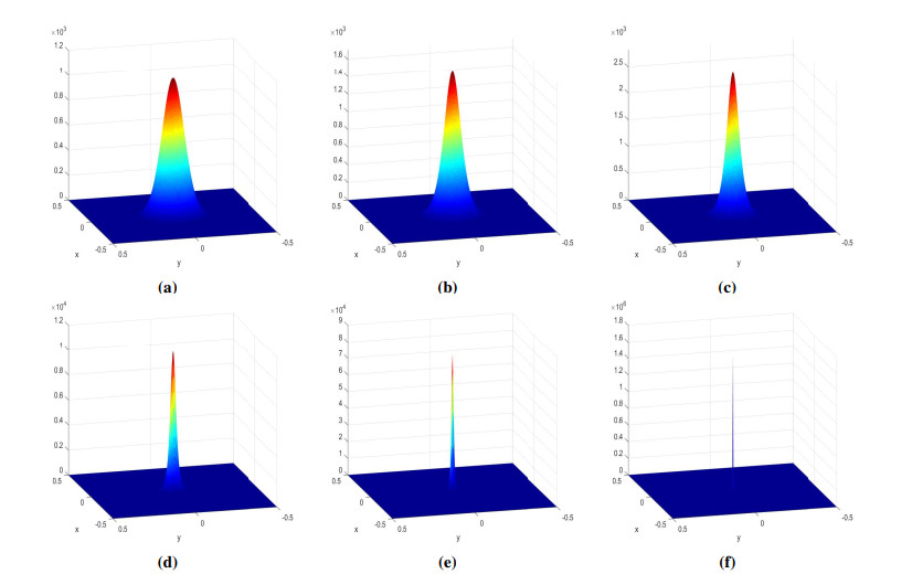
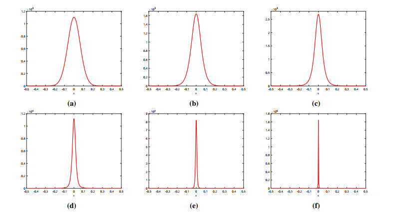
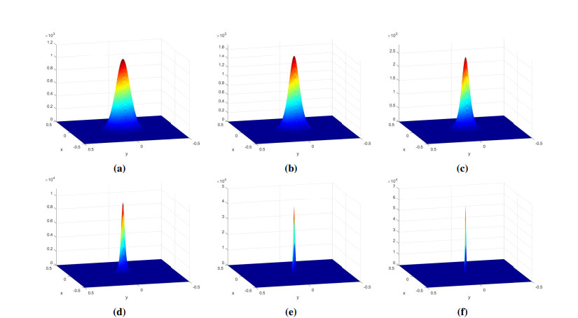
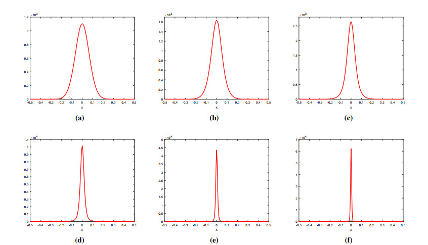
1.   Introduction

In this paper, we focus on the numerical solution of the following Keller-Segel (K-S) chemotaxis model including self- and cross-diffusion terms and a logistic source, i.e.,

with the initial conditions

and Neumann boundary conditions

or Dirichlet boundary conditions

where ${\Omega _t} = \Omega \times (0, T]$ is a given bounded rectangular domain, $\Omega \in$ ${\mathbb{R}^d}\; (d = 1, 2)$, $T > 0$, $\partial \Omega$ is the boundary of $\Omega$, $\mathbf{n}$ is the unit normal vector of $\partial \Omega$, $\mathbf{x}$ represents the space variable and $t$ stands for time variable. $u = u(\mathbf{x}, t)$ represents the cell (or organism) density and $v = v(\mathbf{x}, t)$ denotes the concentration of the chemical signal. The function where $D(u)$ describes the random diffusion rate of the cells, $D(u) = \lambda + \theta u, \lambda, \theta \ge 0$. $\chi(v)$ represents the chemotactic sensitivity function, in this paper, $\chi(v)$ is treated as a positive constant. $u\nabla v$ represents the chemotactic flux of cells. The function $f(u)$ represents the logistic source that describes cell growth and death. We take $f(u) = \delta u(1 - u)$. ${p_1}$, ${p_2}$, $\alpha$ and $\beta$ are positive constants, they are expressed as the diffusivity, the degradation rate and the formation rate of the chemoattractant, respectively. $\alpha u - \beta v$ is a kinetic function that describes the production and degradation of a chemical signal. $\varphi (\mathbf{x}, t)$ and $\psi (\mathbf{x}, t)$ are given smooth functions. In ^[17,25,28], the authors have proved, for arbitrarily small cross diffusion, the global time existence and uniqueness of weak solutions for the K-S chemotaxis model (1.1) through the use of an entropy function such as for $t \to \infty$.

One of the key characteristics of living organisms is that when they are stimulated by external environmental factors ^[1], they make directional movements towards or away from the stimulus. Chemotaxis refers to the directional movement of a cell or microorganism in response to a chemical stimulus along a concentration gradient of the stimulus. Chemotaxis plays an important role in bacterial aggregation, self-organization, and some physiological and pathological processes, such as, bacterial aggregation patterns, slime mold formation, tumor invasion, wound healing, embryonic development and angiogenesis ^[2]. The important properties of Eq (1.1) are the self-aggregation phenomenon and spatial pattern formation. The mathematical model and theory of chemotaxis can be traced back to the pioneering work of Patlak in the 1950s ^[3], as well as Keller and Segel in the 1970s ^[4,5,6]. For an in-depth understanding of the background of chemotaxis models, we can consult Refs. ^{[7,8,9,10,11,12]} and the references therein. It is well known that the solution of Eq (1.1) has great variation. It can develop sharp structures and exhibit finite time blow-up patterns within small regions of the domain ^{[13,14,15,16]}; thus, the numerical solution of the K-S system is challenging. How to avoid the blow-up problem of cells has been researched by many researchers. For example, four methods were mentioned in ^[17]: modify the chemotactic sensitivity, modify the cell diffusion, add a cross-diffusion term in the equation for the chemical signal or consider nonvanishing growth-death models. In the present review, we carefully discuss the K-S chemotaxis system with self- and cross-diffusion terms and a logistic source, as well as its related issues.

The model is a cross-coupled system of time-diffusion-chemotaxis partial differential equations with a complex structure and strong non-linearity, which makes it difficult to obtain an analytical solution. Numerical calculations and simulations play a key role in understanding these cellular dynamics mentioned above. Although a large body of research work in the literature already exists for these models, only a few numerical methods have been proposed; therefore, it is necessary to study effective numerical methods for the modeling and analysis of chemotactic systems. Below we review the previous references for solving the K-S chemotaxis system: Akhmouch and Amine ^[1] discussed a new linearized implicit finite volume method for solving K-S chemotaxis growth models, developed a linearized semi-exponentially fitted scheme and verified it to be first-order convergent. Saito ^[15] established a conservative upwind finite element scheme for the simplified K-S model. The method is the first-order convergent. Sulman and Nguyen ^[18] used an adaptive moving mesh finite element method to study the K-S chemotaxis model, and numerically simulated the finite time blow-up and pattern formation characteristics of the model solution in the boundary and central regions and verified the second-order accuracy of numerical scheme. Qiu et al. ^[19] used the Galerkin method to solve the classical K-S chemotaxis model and developed a fully explicit scheme that has the third-order accuracy in time. Borsche et al. ^[20] used a first-order upwind scheme to solve the one-dimensional (1D) K-S chemotaxis model on general network topologies. Shen and Xu ^[21] proposed first-order and second-order schemes based on the gradient flow structure to solve parabolic-elliptic equations, and they developed a first-order scheme by using convex splitting to solve parabolic-parabolic equations. Braun et al. ^[22] proposed a first-order accuracy in time and second-order accuracy in space scheme for the doubly-parabolic systems at the inner nodes of the network connecting the two-dimensional (2D) chambers with the 1D channels. Xiao et al. ^[23] proposed a new semi-implicit scheme discretization of the characteristic derivative surface for the chemotaxis model using the finite element method with second-order accuracy. Zhang et al. ^[24] proposed a five-step fully implicit compact difference scheme for solving the K-S chemotaxis model. The scheme has fourth-order accuracy in both spatial and temporal directions. Hassan and Harfash ^[25] established a full finite element approximation scheme for the K-S model with self- and cross-diffusion terms and a logistic source, and numerically simulated the explosion phenomenon of high concentration solution of bacteria aggregation. Most of the above numerical methods produce results with low precision, which often leads to large computational errors. If we want to obtain high-resolution computed results to meet the needs of practical problems, we need to compute on very fine grid. In addition, high-order discretization usually needs non-compact stencils, which increases the band-width of the coefficient matrix of the algebraic equations. Both grid refinement and increasing the width of the matrix generate a great number of arithmetic calculations. From this viewpoint, neither the low-order method with fine meshes nor the high-order method with non-compact meshes appear to be computationally cost-effective. This is why high-order compact (HOC) finite difference methods has become important. On the basis of this viewpoint, in this paper, we aim to use the finite difference method to establish HOC difference schemes for Eq (1.1). The truncation error remainder correction method is used to deal with the temporal derivative and the fourth-order Padé compact difference schemes are used to treat the spatial derivatives. It is shown that they yield temporally second-order and spatially fourth-order accuracy.

The rest of this article is designed as follows: Section 2 establishes the difference scheme for 1D K-S chemotaxis models; Section 3 proposes the difference scheme for 2D K-S chemotaxis models. Section 4 verifies the accuracy and reliability of the presented schemes, and it shows the simulation of the blow-up phenomenon and bacterial pattern formation. Section 5 is the conclusion of the whole work.

2.   High-order finite difference scheme for 1D K-S model

First, we consider the 1D model of Eq (1.1) as follows:

with the initial conditions

and Neumann boundary conditions

or Dirichlet boundary conditions

Consider the domain $\left[{{a}, {b}} \right] \times(0, T]$, in which $\left[{{a}, {b}} \right]$ is divided into $M$ uniform intervals, $a = \mathop x\nolimits_0 < \mathop x\nolimits_1 < \mathop x\nolimits_2 < \cdot \cdot \cdot < \mathop x\nolimits_{M} = b$, and $(0, T]$ is divided into $N$ uniform intervals. The spatial step size and temporal step size are $h = \frac{b-a}{M}$ and $\tau = \frac{T}{N}$, respectively.

Denote the mesh points as ($x_i, t_n$), ${x_i} = a + ih, {t_n} = n\tau$, $i = 0, 1, \cdots, M$, $n = 0, 1, \cdots, N$, and denote $\Omega_{\tau} = \{t_n|0\leq n\leq N\}$, $\Omega = \{x_i|0\leq i\leq M\}$, $\Omega_{t} = \Omega\times \Omega_{\tau}$. Then, define grid function $u = \{u_{i}^n|0\leq i\leq M, 0\leq n\leq N\}$, $v = \{v_{i}^n|0\leq i\leq M, 0\leq n\leq N\}$ on $\Omega_{t}$. For convenience, we denote $u_i^n = u(x_i, t_n)$, $v_i^n = v(x_i, t_n), D_i^n = D(u_i^n), f_i^n = f(u_i^n)$.

The difference operator is defined as follows:

We consider the values of Eqs (2.1) and (2.2) at the n-th level of time. By the Taylor expansion for the first-order derivatives in time, it becomes

To construct second-order accuracy scheme in the temporal direction, $u_{tt}$ and $v_{tt}$ in Eqs (2.6) and (2.7) need to be processed. Therefore, we take the derivatives of both sides of Eqs (2.1) and (2.2) with respect to $t$, and get

To discretize Eqs (2.8) and (2.9) at point $(x_i, t_n)$, we use the central difference quotient for the spatial derivatives and forward difference quotient for the temporal derivatives,

and substituting Eqs (2.10) and (2.11) into Eqs (2.6) and (2.7), respectively, then discretizing Eqs (2.1) and (2.2) at point $(x_i, t_n)$, substituting Eqs (2.6) and (2.7) into Eqs (2.1) and (2.2), we obtain

Substituting the definitions of $\delta _t^+$, $\delta _x$ and $\delta _x^2$ into Eqs (2.12) and (2.13), and omitting the truncation error, we get

For the first- and second-order derivatives in Eqs (2.14) and (2.15), we use the following fourth-order compact Padé schemes ^[26],

where $\phi \in {\{D, u, v\}}$, for $i = 1, 2, ..., M - 1$.

Because the values of $({\phi _x})_0^n$, $({\phi _x})_M^n$, $({\phi _{xx}})_0^n$ and $({\phi _{xx}})_M^n$ in Eqs (2.16) and (2.17) are unknown, and the values of $u_0^{n + 1}$, $u_M^{n + 1}$, $v_0^{n + 1}$ and $v_M^{n + 1}$ in Eqs (2.14) and (2.15) are also unknown, they need to be calculated. We discuss this on a case-by-case basis based on boundary conditions as follows.

For the Dirichlet boundary conditions, the values of $u_0^{n + 1}$, $u_M^{n + 1}$, $v_0^{n + 1}$ and $v_M^{n + 1}$ are computed by Eq (2.5). And the values of $({\phi _x})_0^n$, $({\phi _x})_M^n$, $({\phi _{xx}})_0^n$ and $({\phi _{xx}})_M^n$ are calculated by the consistent fourth-order boundary schemes ^[27],

For the Neumann boundary conditions, we use Eq (2.4) directly to calculate the values of $({\phi _x})_0^n$ and $({\phi _x})_M^n$. The values of $({\phi _{xx}})_0^n$ and $({\phi _{xx}})_M^n$ are computed by Eqs (2.20) and (2.21). The values of $u_0^{n + 1}$, $u_M^{n + 1}$, $v_0^{n + 1}$ and $v_M^{n + 1}$ are computed by following fourth-order approximation constructed in ^[24].

where $\eta \in {\{u, v\}}$.

Remark 1: Eqs (2.14) and (2.15) are finite difference schemes after discretization of Eqs (2.1) and (2.2). The schemes involve only three grid points, and the local truncation errors are $O({\tau ^2} + \tau {h^2} + {h^4})$. So the schemes yield the second-order accuracy in time and fourth-order accuracy in space.

The algorithm for solving Eqs (2.1)–(2.4) is described as follows:

Remark 2: The above algorithm is applicable for the 1D K-S chemotaxis model given by Eqs (2.1) and (2.2) with Neumann boundary conditions. In the numerical example, we also use the Dirichlet boundary conditions. It needs to move to Step 2, where the values of $({\phi _x})_0^n$, $({\phi _x})_M^n$, $({\phi _{xx}})_0^n$ and $({\phi _{xx}})_M^n$ are computed by using Eqs (2.18)–(2.21); then, in Step 3, the values of ${\eta}_0^{n + 1}$ and ${\eta}_M^{n + 1}$ are directly computed by using Eq (2.5).

3.   High-order finite difference scheme for 2D K-S model

Then, we consider the 2D K-S model of Eq (1.1) as follows:

with the initial conditions

and Neumann boundary conditions

or Dirichlet boundary conditions

where $D(u)$ and $f(u)$ are similar to the 1D case.

Consider the domain $\left[{{a}, {b}} \right]^2 \times(0, T]$, in which $\left[{{a}, {b}} \right]$ is divided into $M$ uniform intervals, $a = \mathop x\nolimits_0 < \mathop x\nolimits_1 < \mathop x\nolimits_2 < \cdot \cdot \cdot < \mathop x\nolimits_{M} = b$, $a = \mathop y\nolimits_0 < \mathop y\nolimits_1 < \mathop y\nolimits_2 < \cdot \cdot \cdot < \mathop y\nolimits_{M} = b$, and $(0, T]$ is divided into $N$ uniform intervals. The spatial step size and time step size are $h = \frac{b-a}{M}$ and $\tau = \frac{T}{N}$, respectively.

Denote the mesh points as ($x_i, y_j, t_n$), ${x_i} = a + ih, {y_j} = a + jh, {t_n} = n\tau$, $i = 0, 1, \cdots, M$, $j = 0, 1, \cdots, M$, $n = 0, 1, \cdots, N$, and $\Omega_{\tau} = \{t_n|0\leq n\leq N\}$, $\Omega = \{(x_i, y_j)|0\leq i\leq M, 0\leq j\leq M\}$, $\Omega_{t} = \Omega\times \Omega_{\tau}$. Then, define the grid functions $u = \{u_{i, j}^n|0\leq i\leq M, 0\leq j\leq M, 0\leq n\leq N\}$, $v = \{v_{i, j}^n|0\leq i\leq M, 0\leq j\leq M, 0\leq n\leq N\}$ on $\Omega_{t}$. For convenience, we denote $u_{i, j}^n = u(x_i, y_j, t_n)$, $v_{i, j}^n = v(x_i, y_j, t_n), D_{i, j}^n = D(u_{i, j}^n)$ and $f_{i, j}^n = f(u_{i, j}^n)$.

The difference operator is defined as follows:

Similarly, ${\delta _y}u_{i, j}^n$ and $\delta _y^2u_{i, j}^n$ can be defined.

We consider the value of Eq (3.1) at the n-th level of time, use the Taylor expansion for the first-order derivative in time, we get

To gain second-order accuracy in the temporal dimension, $u_{tt}$ in Eq (3.6) needs to be processed. We take the derivative of both sides of Eq (3.1) with respect to $t$, and then we have

To discretize Eq (3.7) at point $(x_i, y_j, t_n)$, we use the forward difference quotient approximation for the time derivatives and central difference quotient approximation for the spatial derivatives, respectively. Then substituting it into Eq (3.6), we have

considering Eq (3.1) at point $(x_i, y_j, t_n)$ and combining with Eq (3.8), we obtain

Similarly, using the same approach for Eq (3.2), we obtain

substituting the definitions of $\delta _t^+$, $\delta _x$, $\delta _y$, $\delta _x^2$ and $\delta _y^2$ into Eqs (3.9) and (3.10), and omitting the truncation error, we have

For the first- and second-order derivatives in Eqs (3.11) and (3.12), we use the following fourth-order Padé schemes ^[26],

where $\phi \in {\{ D, u, v\}}$, and $i, j = 1, 2, ..., M-1$.

The values of $({\phi _x})_{0, j}^n$, $({\phi _x})_{M, j}^n$, $({\phi _y})_{i, 0}^n$, $({\phi _y})_{i, M}^n$, $({\phi _{xx}})_{0, j}^n$, $({\phi _{xx}})_{M, j}^n$, $({\phi _{yy}})_{i, 0}^n$ and $({\phi _{yy}})_{i, M}^n$ are unknown. In addition, the values of $u_{0, j}^{n+1}$, $u_{M, j}^{n+1}$, $u_{i, 0}^{n+1}$, $u_{i, M}^{n+1}$, $v_{0, j}^{n+1}$, $v_{M, j}^{n+1}$, $v_{i, 0}^{n+1}$ and $v_{i, M}^{n+1}$ are also unknown and they need to be calculated. Same with the 1D method, they are discussed according to the boundary conditions.

For the Dirichlet boundary conditions, the values of $u_{0, j}^{n+1}$, $u_{M, j}^{n+1}$, $u_{i, 0}^{n+1}$, $u_{i, M}^{n+1}$, $v_{0, j}^{n+1}$, $v_{M, j}^{n+1}$, $v_{i, 0}^{n+1}$ and $v_{i, M}^{n+1}$ are computed by using Eq (3.5), and the values of $({\phi _x})_{0, j}^n$, $({\phi _x})_{M, j}^n$, $({\phi _y})_{i, 0}^n$, $({\phi _y})_{i, M}^n$, $({\phi _{xx}})_{0, j}^n$, $({\phi _{xx}})_{M, j}^n$, $({\phi _{yy}})_{i, 0}^n$ and $({\phi_{yy}})_{i, M}^n$ are computed with the consistent fourth-order boundary schemes ^[27].

in which $i, j = 0, 1, 2, ..., M$.

For the Neumann boundary conditions, we can directly use Eq (3.4) to valuate $({\phi _x})_{0, j}^n$, $({\phi _x})_{M, j}^n$, $({\phi _y})_{i, 0}^n$ and $({\phi _y})_{i, M}^n$, and use Eqs (3.21) and (3.24) to compute $({\phi _{xx}})_{0, j}^n$, $({\phi _{xx}})_{M, j}^n$, $({\phi _{yy}})_{i, 0}^n$ and $({\phi _{yy}})_{i, M}^n$. The values of $u_{0, j}^{n+1}$, $u_{M, j}^{n+1}$, $u_{i, 0}^{n+1}$, $u_{i, M}^{n+1}$, $v_{0, j}^{n+1}$, $v_{M, j}^{n+1}$, $v_{i, 0}^{n+1}$ and $v_{i, M}^{n+1}$ are evaluated by the following fourth-order schemes constructed in ^[24].

in which $\eta \in {\{u, v\}}$, $i, j = 0, 1, 2, ..., M$.

Remark 3: Equations (3.11) and (3.12) are finite difference schemes after discretization of Eqs (3.1) and (3.2). It is easy to find that the schemes are only involved in five grid points, and that the local truncation errors of Eqs (3.11) and (3.12) are $O({\tau ^2} + \tau {h^2}+ {h^4})$, i.e., the scheme has second-order accuracy in time direction and fourth-order accuracy in space direction.

The algorithm for solving Eqs (3.1)–(3.4) is described in Algorithm 2.

Remark 4: The above algorithm is described for the 2D K-S chemotaxis model (3.1) and (3.2) with Neumann boundary conditions. In the numerical example, we are also going to use Dirichlet boundary conditions. It needs to compute the values of $({\phi _x})_{0, j}^n$, $({\phi _x})_{M, j}^n$, $({\phi _y})_{i, 0}^n$ and $({\phi _y})_{i, M}^n$ with Eqs (3.17)–(3.24) in the Step 2, and the values of ${\eta}_{0, j}^{n+1}$, ${\eta}_{M, j}^{n+1}$, ${\eta}_{i, 0}^{n+1}$ and ${\eta}_{i, M}^{n+1}$ are calculated by Eq (3.5) in the Step 3.

4.   Numerical experiments

In this section, we employ several numerical examples to verify the performances of the proposed method for solving the K-S chemotaxis system give by Eqs (1.1)–(1.4). We verify the accuracy of the numerical solution of the K-S chemotaxis model with Dirichlet boundary conditions in 1D and 2D, and we compare it with the results in existing literature. We also study the numerical solution of the K-S chemotaxis model with Neumann boundary conditions in 2D.

To measure accuracy, we simply modify the problem Eq (1.1) by adding the source terms $s(\mathbf{x}, t)$ and $g(\mathbf{x}, t)$ and transform it into the following equations:

The computations are programmed in Fortran 77 language with double precision arithmetic and are implemented on a personal computer equipped with Intel Core i7-7500U CPU @ 2.70 GHz 2.90 GHz, 4.00 GB RAM Windows workstation. The convergence rate of errors are defined as follows:

where, $p$ could be $\infty$ or 2. $||e_{h}^{u}||_2 = \!\sqrt {h\!\sum\limits_{i = 0}^M {{{[U({x_i}, {t_N})-u({x_i}, {t_N})]}^2}}}\!$, $||e_{h}^{v}||_2 = \sqrt {h\sum\limits_{i = 0}^M {{{[V({x_i}, {t_N})-v({x_i}, {t_N})]}^2}} }\!$, $||e_{h}^{u}||_\infty = \mathop {\max }\limits_{0 \le i \le M} |U({x_i}, {t_N}) - u({x_i}, {t_N})|$ and $||e_{h}^{v}||_\infty = \mathop {\max }\limits_{0 \le i \le M} |V({x_i}, {t_N}) - v({x_i}, {t_N})|$ for 1D. $||e_{h}^{u}||_2 = \!\sqrt {{h^2}\!\sum\limits_{i, j = 0}^{{M}} { {{{[U({x_i}, {y_j}, {t_N})-u({x_i}, {y_j}, {t_N})]}^2}} } }\!$, $||e_{h}^{v}||_2 = \!\sqrt {{h^2}\!\sum\limits_{i, j = 0}^{{M}} { {{{[V({x_i}, {y_j}, {t_N})-v({x_i}, {y_j}, {t_N})]}^2}} } }\!$, $||e_h^u|{|_\infty } = \mathop {\max }\limits_{0 \le i,j \le M} |U({x_i},{y_j},{t_N}) - u({x_i},{y_j},{t_N})|$ and $||e_h^v|{|_\infty } = \mathop {\max }\limits_{0 \le i,j \le M} |V({x_i},{y_j},{t_N}) - v({x_i},{y_j},{t_N})|$ for 2D. $u(x_i, t_N)$, $v(x_i, t_N)$, $u(x_i, y_j, t_N)$ and $v(x_i, y_j, t_N)$ represent the numerical solutions at points $(x_i, t_N)$ and $(x_i, y_j, t_N)$, $U({x_i}, {t_N})$, $V({x_i}, {t_N})$, $U({x_i}, {y_j}, {t_N})$ and $V({x_i}, {y_j}, {t_N})$ represent the exact solutions at points $(x_i, t_N)$ and $(x_i, y_j, t_N)$.

4.1.   Problem 1 ^[25]

First, we consider the 1D K-S chemotaxis model as follows:

where

and

with the initial conditions

and boundary conditions

The exact solutions are $u(x, t) = {e^{ - t + x}}$ and $v(x, t) = {e^{ - t + {x^2}}}.$

To verify the accuracy of the 1D scheme, i.e., Eqs (2.14) and (2.15), we chose an example with an exact solution. Table 3 and Table 4 show the $||e_{h}||_2$ and $||e_{h}||_\infty$ values of numerical solutions $u$ and $v$ using the scheme proposed in this paper and comparisons with the results in ^[25] with different values of $N$ in 1D, with $\tau = 0.1{h^2}, Tol = {10^{{\rm{ - 12}}}}$ for Problem 1. We have used the same problem parameters as ^[25], i.e., $T = 1$, $\delta = \chi = 1$, $\Omega = [0, 1]$ for comparison. From data in Tables 3 and 4, we can see that the convergence order of the difference scheme in this paper reaches the fourth-order in space, which is higher than the method in ^[25]. To satisfy the stability conditions of the scheme in this paper, we have used $\tau {\rm{ = }}0.1{h^2}$ and in ^[25], it was $\tau = 10^{-6}$. It means that we used a larger time step size than that used in ^[25]. The advantage of our method is that we calculate fewer layers of time to reach the same time moment. Therefore, the present compact method can accurately predict the solution of the 1D K-S model.

4.2.   Problem 2 ^[25]

Then, consider the following 2D K-S chemotaxis model:

where

and

with the initial conditions

and boundary conditions

The exact solutions are $u(x, y, t) = {e^{-t+x+y}}$ and $v(x, y, t) = {e^{-t+{x^2}+{y^2}}}.$

Similarly, to test the accuracy of the scheme for the 2D cases, we also chose an example with an exact solution in ^[25]. Tables 5 and 6 list the $||e_{h}||_2$, $||e_{h}||_\infty$ and convergence orders given by the scheme of ^[25] and the presented scheme. We set $Tol = {10^{{\rm{ - 11}}}}$, and the time step $\tau = 0.1{h^2}$. We fix the values of the problem parameters same as that in ^[25]: $T = 1$, $\delta = \chi = 1$. From Tables 5 and 6, we can clearly see that the proposed scheme achieves approximately fourth-order convergence in space. By comparing the results in Tables 5 and 6, we find the computational results in this paper are more accurate than those in ^[25], both in the case of $||e_{h}||_2$ and in the case of $||e_{h}||_\infty$. In addition, we take $\tau = 0.1{h^2}$ to satisfy the stability conditions of the scheme in this paper, while $\tau = 10^{-7}$ was used in ^[25]. Namely, we use a larger time step size than that in the ^[25], but the numerical results we calculated at the same $N$ are better than those in ^[25].

4.3.   Problem 3 ^[25]

Next, we consider the following 2D K-S chemotaxis model with a logistic source.

The initial values of this problem are

with homogeneous Neumann boundary conditions.

To further verify the effectiveness of the proposed finite difference method for 2D K-S chemotaxis models, we used $(x, y) \in {[-1/2, 1/2]}, \tau = {10^{ - 7}}, Tol = {10^{ - 12}}$ for Problem 3. For this problem, the exact solution is not available. Reference ^[14] proved in theory that the solutions would blow-up in a finite time, but the blow-up solution is difficult to capture. The computed results were obtained by the presented difference schemes and compared with those in ^[25]. The approximated solutions of the cell density $u$ at $N = 300, T = {10^{ - 6}}, 5 \times {10^{ - 6}}, {10^{ - 5}}, 2.5 \times {10^{ - 5}}, 5 \times {10^{ - 5}}$ and $8 \times {10^{ - 5}}$ are plotted in Figure 1. The corresponding slices along $y = 0$ of approximated cell density $u$ are plotted in Figure 2. We find that as time increases the phenomenon of the peak becomes more and more obvious. We observe that the blow-up time is the same as the conjecture in ^[25].

The approximated solution of the cell density $u$ at $N = 150, T = {10^{ - 6}}, N = 150, T = 5 \times {10^{ - 6}}, N = 150, T = {10^{ - 5}}, N = 200, T = 2.5 \times {10^{ - 5}}, N = 200, T = 5 \times {10^{ - 5}}$ and $N = 300$, $T = {8 \times10^{ - 5}}$ are plotted in Figure 3. The corresponding slices along $y = 0$ of the approximation of the cell density $u$ are plotted Figure 4.

Through the experiment, we find that a negative cell density $u$ may occur for different values of $N$ at the same time, which is unreasonable. In order to preserve the positivity of the cell density $u$, for time smaller than $T = 5 \times {10^{ - 5}}$, we applied $N = 150$, and for time values larger than $T = 5 \times {10^{ - 5}}$, we applied $N = 300$. It has a peak in the center of the domain $\Omega$, where the blow-up of the cell density $u$ occurs in finite time. As the number of mesh points increases, the change in the accuracy of the solution becomes not significant ^[25].

By comparison of $\delta = 0$ and $\delta = 1$, we can clearly see from Figures 2d–f and Figures 4d–f that when $\delta = 1$, the value of the cell density $u$ decreases significantly. For further comparison, variation of the maximum value of approximated cell density $u$ with time $t$ when $\delta = 0$ and $\delta = 1$ is plotted in Figure 5. We note that in Figure 5a, when $\delta = 0$ the value of approximated cell density $u$ at time $8.24e-05$ is $3.72e+08$, the value at this moment is very large and the gradient around it varies considerably. However, in Figure 5b, the value of approximated cell density $u$ is $6.15e+04$ compared to that with $\delta = 0$, which is significantly smaller. It is verified that the logical source term can avoid the blow-up, that is, the logical source term is important for the model. This point is consistent with the fourth-order method for the cells to avoid the blow-up problems mentioned in ^[17].

4.4.   Problem 4 ^[1]

Finally, we consider the following 2D chemotaxis growth model for bacterial pattern formation ^[31] with homogeneous Neumann boundary conditions,

with the initial values

and $v(x, y, 0) = 1/32$.

The term $2u(1 - u)$ is a logistic source representing the growth rate of $u$. For this model, the computational domain is the square $\Omega = (-8, 8)^2$, since the model is quite sensitive to the choice of the parameters, we applied the values of the parameters to be the same as in ^[1]: $D = 0.0625$, $\chi = 6$, $\beta = 16$. To understand the evolution of the solution, we take $T = 1, 5, 10, 30$, where $rand$ is a random perturbation which is a constant between 0 and 1 on each cell of the mesh and $||x||_2$ denotes the Euclidean distance to the center node $(0, 0, 0)$ of the domain $\Omega$. The time step $\tau = 10^{-5}$ was chosen. Figure 6 describes approximate solution of $u$ for $N = 100$ at different times. As we notice from Figure 6, the initial concentration of the cell $u$ slowly expands from the center to the boundaries of the domain $\Omega$ with a periodic form of continuous rings. The behavior of our calculated solution is consistent with that simulated in ^[1].

5.   Conclusions

Based on the fourth-order Padé compact difference schemes for the spatial derivatives and the truncation error remainder correction method for the temporal derivative, we have proposed a highly accurate numerical scheme based on the finite difference method to solve the K-S chemotaxis system with self- and cross-diffusion terms and a logistic source in 1D and 2D. The local truncation errors of the schemes are $O({\tau ^2} + \tau {h^2}+ {h^4})$, which means that the schemes yield temporally second-order and spatially fourth-order accuracy. The accuracy and effectiveness of the 1D and 2D schemes have been verified by numerical examples. Moreover, we simulated the blow-up phenomenon and bacterial pattern formation of K-S chemotaxis model (1.1) by using the presented numerical method.

We note that positivity preserving nature of numerical methods for K-S chemotaxis models is a very important aspect, which was not taken into account in this paper. We will consider it in our ongoing work. Meanwhile, the three-dimensional (3D) K-S chemotaxis model has been numerically studied by some researchers ^[29,30]. Zhao et al. ^[29] investigated the improved Petrov-Galerkin finite element method defined on general static surfaces. A semi-implicit second-order scheme based on gradient and Laplace recoveries has been used to obtain a completely discrete form. Huang et al. ^[30] used the operator-splitting finite-element method combined with the flux-corrected transport algorithm to solve the 3D chemotaxis model. The method, which is used to solve several 1D sub-problems can keep the numerical solution non-negative. The scheme has second-order accuracy in the spatial direction. We are trying to extend the present method to the 3D K-S chemotaxis model. This work is in progress and the research results will be reported in the near future.

Use of AI tools declaration

The authors declare they have not used Artificial Intelligence (AI) tools in the creation of this article.

Acknowledgments

This work was partially supported by the National Natural Science Foundation of China (12161067, 11961054), Natural Science Foundation of Ningxia (2022AAC02023), National Youth Top-notch Talent Support Program of Ningxia, and Graduate Innovation Program of Ningxia University (CXXM2022-12).

Conflict of interest

The authors declare that there is no conflict of interest.