We investigate the homogenization of inclusions of infinite conductivity, randomly stationary distributed inside a homogeneous conducting medium. A now classical result by Zhikov shows that, under a logarithmic moment bound on the minimal distance between the inclusions, an effective model with finite homogeneous conductivity exists. Relying on ideas from network approximation, we provide a relaxed criterion ensuring homogenization. Several examples not covered by the previous theory are discussed.
Citation: David Gérard-Varet, Alexandre Girodroux-Lavigne. Homogenization of stiff inclusions through network approximation[J]. Networks and Heterogeneous Media, 2022, 17(2): 163-202. doi: 10.3934/nhm.2022002
We investigate the homogenization of inclusions of infinite conductivity, randomly stationary distributed inside a homogeneous conducting medium. A now classical result by Zhikov shows that, under a logarithmic moment bound on the minimal distance between the inclusions, an effective model with finite homogeneous conductivity exists. Relying on ideas from network approximation, we provide a relaxed criterion ensuring homogenization. Several examples not covered by the previous theory are discussed.

| [1] |
Ergodic theorems for superadditive processes. J. Reine Angew. Math. (1981) 323: 53-67. 
|
| [2] |
H. Ammari, P. Garapon, H. Kang and H. Lee, Effective viscosity properties of dilute suspensions of arbitrarily shaped particles, Asymptot. Anal., 80 (2012) 189–211. |
| [3] |
G. Berkolaiko and P. Kuchment, Introduction to Quantum Graphs, American Mathematical Soc., 2013. |
| [4] |
Network approximation for effective viscosity of concentrated suspensions with complex geometry. SIAM J. Math. Anal. (2005) 36: 1580-1628.
|
| [5] |
Fictitious fluid approach and anomalous blow-up of the dissipation rate in a two-dimensional model of concentrated suspensions. Arch. Ration. Mech. Anal. (2009) 193: 585-622.
|
| [6] |
Network approximation in the limit of small interparticle distance of the effective properties of a high-contrast random dispersed composite. Arch. Ration. Mech. Anal. (2001) 159: 179-227.
|
| [7] |
L. Berlyand, A. G Kolpakov and A. Novikov, Introduction to the Network Approximation Method for Materials Modeling, Cambridge University Press, 148, 2013. |
| [8] |
Increase and decrease of the effective conductivity of two phase composites due to polydispersity. J. Stat. Phys. (2005) 118: 481-509.
|
| [9] |
Error of the network approximation for densely packed composites with irregular geometry. SIAM Journal on Mathematical Analysis (2002) 34: 385-408.
|
| [10] |
Strong and weak blow-up of the viscous dissipation rates for concentrated suspensions. Journal of Fluid Mechanics (2007) 578: 1-34.
|
| [11] |
B. Blaszczyszyn, Lecture notes on random geometric models. random graphs, point processes and stochastic geometry, 2017. |
| [12] |
B. Bollobás, Modern Graph Theory, Springer-Verlag, New York, 1998. |
| [13] |
Network approximation for transport properties of high contrast materials. SIAM J. Appl. Math. (1998) 58: 501-539.
|
| [14] |
Nonlinear stochastic homogenization. Ann. Mat. Pura Appl. (1986) 144: 347-389.
|
| [15] |
M. Duerinckx, Effective viscosity of random suspensions without uniform separation, arXiv: 2008.13188. |
| [16] |
Corrector equations in fluid mechanics: Effective viscosity of colloidal suspensions. Arch. Ration. Mech. Anal. (2021) 239: 1025-1060.
|
| [17] |
M. Duerinckx and A. Gloria, On Einstein's effective viscosity formula, arXiv: 2008.03837. |
| [18] |
M. Duerinckx and A. Gloria, Continuum percolation in stochastic homogenization and the effective viscosity problem, arXiv: 2108.09654. |
| [19] |
D. Gérard-Varet, Derivation of the Batchelor-Green formula for random suspensions, Journal de Mathématiques Pures et Appliquées, 152 (2021), 211–250. |
| [20] |
Analysis of the viscosity of dilute suspensions beyond Einstein's formula. Arch. Ration. Mech. Anal. (2020) 238: 1349-1411.
|
| [21] |
Mild assumptions for the derivation of Einstein's effective viscosity formula. Communications in Partial Differential Equations (2021) 46: 611-629.
|
| [22] |
D. Gérard-Varet and A. Mecherbet, On the correction to Einstein's formula for the effective viscosity, arXiv: 2004.05601. |
| [23] |
L. Giovanni, A First Course in Sobolev Spaces, American Mathematical Society, Providence, RI, 2017. |
| [24] |
The Effective conductivity of densely packed high contrast composites with inclusions of optimal shape. Continuum Models and Discrete Systems (2004) 158: 63-74.
|
| [25] |
A proof of Einstein's effective viscosity for a dilute suspension of spheres. SIAM Journal on Mathematical Analysis (2012) 44: 2120-2145.
|
| [26] |
Effective viscosity of a polydispersed suspension. Journal de Mathématiques Pures et Appliquées. Neuvième Série (2020) 138: 413-447.
|
| [27] |
V. V. Jikov, S. M. Kozlov and O. A. Oleinik, Homogenization of Differential Operators, Springer-Verlag, Berlin Heidelberg, 1994. |
| [28] |
A theorem on the conductivity of a composite medium. Journal of Mathematical Physics (1964) 5: 548-549.
|
| [29] |
S. Mischler, An introduction to evolution PDEs, (2017). |
| [30] |
A local version of Einstein's formula for the effective viscosity of suspensions. SIAM J. Math. Anal. (2020) 52: 2561-2591.
|
| [31] |
E. M. Stein, Singular Integrals and Differentiability Properties of Functions, Princeton University Press, 1994. |


Figures(7)
David Gérard-Varet, Alexandre Girodroux-Lavigne. Homogenization of stiff inclusions through network approximation[J]. Networks and Heterogeneous Media, 2022, 17(2): 163-202. doi: 10.3934/nhm.2022002

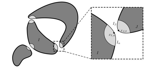
Geometry of the inclusions with a close-up on a gap
Spherical set up. The graph obtained with the whites lines is isomorphic to the multigraph of inclusions
Two inclusions configuration, shorted on the right
Cycle-free configuration set up
On the left, all clusters are far away from the others. On the right, groups of inclusions joined by a grey line form a short
Separation of the domain
Geometry of the gap


 DownLoad: