A 2-dimensional shape optimization problem for tree branches

Alberto Bressan; Sondre Tesdal Galtung; Alberto Bressan; Sondre Tesdal Galtung

doi:10.3934/nhm.2020031

Networks and Heterogeneous Media

2021, Volume 16, Issue 1: 1-29. doi: 10.3934/nhm.2020031

Previous Article Next Article

A 2-dimensional shape optimization problem for tree branches

Alberto Bressan ^{1
,
,},
Sondre Tesdal Galtung ^{2
,}

1.
Department of Mathematics, Penn State University, University Park, PA 16802, USA
2.
Department of Mathematical Sciences, NTNU – Norwegian University of Science and Technology, NO-7491 Trondheim, Norway

Received: 01 June 2020 Revised: 01 September 2020 Published: 30 October 2020
49Q10, 49Q20

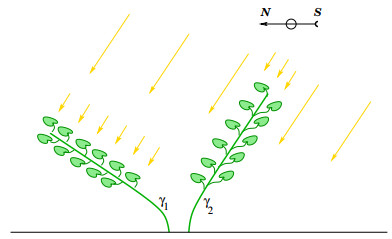
The paper is concerned with a shape optimization problem, where the functional to be maximized describes the total sunlight collected by a distribution of tree leaves, minus the cost for transporting water and nutrient from the base of trunk to all the leaves. In a 2-dimensional setting, the solution is proved to be unique and explicitly determined.

Keywords:

Citation: Alberto Bressan, Sondre Tesdal Galtung. A 2-dimensional shape optimization problem for tree branches[J]. Networks and Heterogeneous Media, 2021, 16(1): 1-29. doi: 10.3934/nhm.2020031

Related Papers:

[1]	Linglong Du, Min Yang . Pointwise long time behavior for the mixed damped nonlinear wave equation in $ \mathbb{R}^n_+ $. Networks and Heterogeneous Media, 2021, 16(1): 49-67. doi: 10.3934/nhm.2020033
[2]	Linglong Du . Long time behavior for the visco-elastic damped wave equation in $\mathbb{R}^n_+$ and the boundary effect. Networks and Heterogeneous Media, 2018, 13(4): 549-565. doi: 10.3934/nhm.2018025
[3]	Hantaek Bae . On the local and global existence of the Hall equations with fractional Laplacian and related equations. Networks and Heterogeneous Media, 2022, 17(4): 645-663. doi: 10.3934/nhm.2022021
[4]	Günter Leugering, Sergei A. Nazarov, Jari Taskinen . The band-gap structure of the spectrum in a periodic medium of masonry type. Networks and Heterogeneous Media, 2020, 15(4): 555-580. doi: 10.3934/nhm.2020014
[5]	Seung-Yeal Ha, Gyuyoung Hwang, Hansol Park . Emergent behaviors of Lohe Hermitian sphere particles under time-delayed interactions. Networks and Heterogeneous Media, 2021, 16(3): 459-492. doi: 10.3934/nhm.2021013
[6]	Arianna Giunti . Convergence rates for the homogenization of the Poisson problem in randomly perforated domains. Networks and Heterogeneous Media, 2021, 16(3): 341-375. doi: 10.3934/nhm.2021009
[7]	Francesca Alessio, Piero Montecchiari, Andrea Sfecci . Saddle solutions for a class of systems of periodic and reversible semilinear elliptic equations. Networks and Heterogeneous Media, 2019, 14(3): 567-587. doi: 10.3934/nhm.2019022
[8]	Ciro D'Apice, Olha P. Kupenko, Rosanna Manzo . On boundary optimal control problem for an arterial system: First-order optimality conditions. Networks and Heterogeneous Media, 2018, 13(4): 585-607. doi: 10.3934/nhm.2018027
[9]	María Anguiano, Francisco Javier Suárez-Grau . Newtonian fluid flow in a thin porous medium with non-homogeneous slip boundary conditions. Networks and Heterogeneous Media, 2019, 14(2): 289-316. doi: 10.3934/nhm.2019012
[10]	Wen Shen . Traveling waves for conservation laws with nonlocal flux for traffic flow on rough roads. Networks and Heterogeneous Media, 2019, 14(4): 709-732. doi: 10.3934/nhm.2019028

Abstract

1. Introduction

In this paper, we study the pointwise long time behavior of the solution for the nonlinear wave equation with frictional and visco-elastic damping terms

$\begin{align} \begin{aligned} \left\{\begin{array}{lll} \partial_{t}^2u- c^2\Delta u+\nu_1\partial_tu-\nu_2\partial_t\Delta u = f(u),\\ u|_{t = 0} = u_0({\bf{x}}),\\ u_t|_{t = 0} = u_1({\bf{x}}),\end{array}\right. \label{{1.1}} \end{aligned} \end{align}$

(1)

in multi-dimensional half space $\mathbb{R}^n_+: = \mathbb{R}_+\times \mathbb{R}^{n-1}$ , with absorbing and radiative boundary condition

$\begin{align} \begin{aligned} \left(a_{1}\partial_{x_1}u+a_{2}u\right)(x_1 = 0,{\bf{x'}},t ) = 0. \label{{1.2}} \end{aligned} \end{align}$

(2)

${\bf{x}} = (x_1, {\bf{x}}')$ is the space variable with $x_1\in \mathbb{R}_+: = (0,\infty)$ , ${\bf{x'}} = (x_2,\cdots, x_n)\in\mathbb{R}^{n-1}$ , $t>0$ is the time variable. $\nu_1$ and $\nu_2$ are positive constant viscosities, $a_1$ and $a_2$ are constants. The Laplacian $\Delta = \sum_{j = 1}^n\partial_{x_j}^2$ , $f(u)$ is the smooth nonlinear term and $f(u) = O(|u|^k)$ when $k>0$ .

Over the past few decades, many mathematicians have concentrated on solving different kinds of damped nonlinear wave equations. The first kind is called the frictional damped wave equation, which is given as follows

$\begin{align} \begin{aligned} \left\{\begin{array}{lll} \partial_{t}^2u- c^2\Delta u+\nu\partial_t u = f(u),\\ u|_{t = 0} = u_0({\bf{x}}),\\ u_t|_{t = 0} = u_1({\bf{x}}),\end{array}\right. \label{{1.10}} \end{aligned} \end{align}$

(3)

see [9,19,20,23] for the references. It is showed that for the long time, the fundamental solution for the linear system of (3) behaves like the Gauss kernel $\frac{e^{-\frac{|{\bf{x}}|^2}{C(t+1)}}}{(t+1)^{\frac{n}{2}}}$ . The second kind is called the visco-elastic damped wave, which is given by the following

$\begin{align} \begin{aligned} \left\{\begin{array}{lll} \partial_{t}^2u- c^2\Delta u-\nu\partial_t \Delta u = f(u),\\ u|_{t = 0} = u_0({\bf{x}}),\\ u_t|_{t = 0} = u_1({\bf{x}}).\end{array}\right. \label{{1.10a}} \end{aligned} \end{align}$

(4)

One can refer to [22] for the decaying rate of the linear solution, [11,12] for the asymptotic profiles of the linear problem, [4,21] for the nonlinear equation, etc. In [9], the authors studied the fundamental solution for the linear system of (4). The results show that the hyperbolic wave transport mechanism and the visco-elastic damped mechanism interact with each other so that the solution behaves like the convented heat kernel, i.e., $\frac{e^{-\frac{(|{\bf{x}}|-ct)^2}{C(t+1)}}}{(t+1)^{\frac{3n-3}{4}}}$ for the odd dimensional case and $\frac{e^{-\frac{(|{\bf{x}}|-ct)^2}{C(t+1)}}}{(t+1)^{\frac{3n-1}{4}}}+\frac{H(ct-|{\bf{x}}|)}{(1+t)^{\frac{3n-2}{4}}(ct-|{\bf{x}}|+\sqrt{t})^{\frac{1}{2}}}$ for the even dimensional case. The solution exhibits the generalized Huygens principle. For other damped wave equations, one can refer to [2,27] for the damped abstract wave equation, and [14,15,16] for the existence and large time behavior of the solutions for the Cauchy problem of mixed damping (both frictional and visco-elastic damping terms are involved) wave equation.

For the initial-boundary value problem of the different damped wave equations, many authors studied the global well-posedness existence, long time behaviors, global attractors and decaying rate estimates of some elementary wave by using delicate energy estimate method, for example [1,13,25,26,28,29]. In this paper, we will use the pointwise estimate technique to give the long time behavior of the solution for system (1) with boundary condition (2). The main part of this technique is the construction and estimation of the Green's functions for the following linear systems:

$\begin{align} \begin{aligned} \left\{\begin{array}{lll} \partial_{t}^2\mathbb{G}_1-c^2\Delta\mathbb{G}_1+\nu_1\partial_t \mathbb{G}_1-\nu_2\partial_t\Delta \mathbb{G}_1 = 0, x_1,y_1 > 0,{\bf{x'}}\in \mathbb{R}^{n-1},\quad t > 0,\\ \mathbb{G}_1\left(x_1,{\bf{x'}}, 0;y_1\right) = \delta(x_1-y_1)\delta({\bf{x'}}), {\mathbb{G}_1}_t\left(x_1,{\bf{x'}}, 0;y_1\right) = 0,\\ a_{1}\partial_{x_1}\mathbb{G}_1(0,{\bf{x'}},t;y_1)+a_{2}\mathbb{G}_1(0,{\bf{x'}},t;y_1) = 0; \end{array}\right. \label{{1.8}} \end{aligned} \end{align}$

(5)

$\begin{align} \begin{aligned} \left\{\begin{array}{lll} \partial_{t}^2\mathbb{G}_2-c^2\Delta \mathbb{G}_2+\nu_1\partial_t \mathbb{G}_2-\nu_2\partial_t\Delta \mathbb{G}_2 = 0, x_1,y_1 > 0,{\bf{x'}}\in \mathbb{R}^{n-1}, \quad t > 0,\\ \mathbb{G}_2\left(x_1,{\bf{x'}}, 0;y_1\right) = 0, {\mathbb{G}_2}_t\left(x_1,{\bf{x'}}, 0;y_1\right) = \delta(x_1-y_1)\delta({\bf{x'}}),\\ a_{1}\partial_{x_1}\mathbb{G}_2(0,{\bf{x'}},t;y_1)+a_{2}\mathbb{G}_2(0,{\bf{x'}},t;y_1) = 0. \end{array}\right. \label{{1.8a}} \end{aligned} \end{align}$

(6)

The way of estimating the Green's functions $\mathbb{G}_i$ was initiated by [17] and developed by [3,5,6,8,10,18,24] and the reference therein. Following the scheme in [10], we will find the relations between the fundamental solutions for the linear Cauchy problem and Green's functions for the linear half space problem, by comparing their symbols in the transformed tangential-spatial and time variables. Then the Green's functions can be described in terms of the fundamental solutions and the boundary surface operator.

With the help of the accurate expression of Green's functions for the linear half space problem and the Duhamel's principle, we get the pointwise long time behavior for the nonlinear solution $\partial_{{\bf{x}}}^{\alpha}u$ , $|\alpha|\le1$ . We only treat the case $a_1a_2<0$ . The boundary condition of Dirichlet type ( $a_1 = 0$ ) and Neumann type ( $a_2 = 0$ ) are much simpler. For the case of $a_1a_2>0$ , the linear problem is unstable. The main results of our paper are given as follows:

Theorem 1.1. Let $n = 2,3$ be the spatial dimension, $k>1+\frac{2}{n}$ . Assume the initial data $(u_0({\bf{x}}), u_1({\bf{x}}))\in (H^{l+1}\cap W^{l,1})\times (H^{l}\cap W^{l,1})$ , $l\ge[\frac{n}{2}]+2$ , and satisfy

$\begin{align*} \begin{aligned} |\partial_{{\bf{x}}}^{\alpha}u_0, \partial_{{\bf{x}}}^{\alpha}u_1|\le O(1)\varepsilon(1+|{\bf{x}}|^2)^{-r}, \ \ r > \frac{n}{2}, \ \ |\alpha|\le 1, \end{aligned} \end{align*}$

$\varepsilon$ sufficiently small, then there exists a unique global classical solution to the problem (1) with the mixed boundary condition (2) while $a_{1}a_{2}\le0$ . The solution has the following pointwise estimate:

$\begin{align*} \begin{aligned} &&|\partial_{{\bf{x}}}^{\alpha}u({\bf{x}},t)| \leq O(1)\varepsilon(1+t)^{-|\alpha|/2}\left(1+t+|{\bf{x}}|^2\right)^{-\frac{n}{2}}. \end{aligned} \end{align*}$

Moreover, we get the following optimal $L^p(\mathbb{R}^n_+)$ estimate of the solution

$\begin{align*} \begin{aligned} \left\|\partial_{{\bf{x}}}^{\alpha}u(\cdot,t)\right\|_{L^p(\mathbb{R}^n_+)}\leq O(1)\varepsilon(1+t)^{-\frac{n}{2}(1-\frac{1}{p})-\frac{|\alpha|}{2}},\ \ p\in(1,\infty]. \end{aligned} \end{align*}$

Remark 1. We can develop a similar theorem for the case of higher space dimension with a suitable choice of $k$ which guarantees the existence of the solution. In Section 2.2, the approximation used in the calculation of the singular part depends on the space dimension. One could modify the short wave part expression of Green's functions for the linear half space problem to prove the results for the general case.

Notations. Let $C$ and $O(1)$ be denoted as generic positive constants. For multi-indices $\alpha = (\alpha_1, \cdots, \alpha_n)$ , $\partial_{{\bf{x}}}^\alpha = \partial_{x_1}^{\alpha_1}\cdots\partial_{x_n}^{\alpha_n}$ , $|\alpha| = \sum_{i = 1}^n\alpha_i$ . Let $L^p$ denotes the usual $L^p$ space on ${\bf{x}}\in\mathbb{R}^n_+$ . For nonnegative integer $l$ , we denote by $W^{l,p} (1\le p<\infty)$ the usual $L^p-$ Soblev space of order $l$ : $W^{l,p} = \{u\in L^p:\partial_{{\bf{x}}}^{\alpha}u\in L^p(|\alpha|\le l)\}(l\ge 1), W^{0,p} = L^p.$ The norm is denoted by $\|\cdot\|_{W^{l,p}} =$ $\|u\|_{W^{l,p}} = \sum_{|\alpha|\le l}\| \partial_{{\bf{x}}}^{\alpha}u \|_{L^p}$ . When $p = 2$ , we define $W^{l,2} = H^l$ for all $l\ge 0$ . We denote $\mathcal{D}_{\delta}: = \{{\boldsymbol{\xi}}\in \mathbb{C}^n| |Im(\xi_i)|\le\delta, i = 1,2,\cdots,n\}$ . Introduce the Fourier transform and Laplace transform of $f({\bf{x}},t)$ as follows:

$\begin{align*} \begin{aligned} &&f({\boldsymbol{\xi}}, t)&: = \mathcal{F}[f]({\boldsymbol{\xi}},t) = \int_{ \mathbb{R}^n}e^{-i{\boldsymbol{\xi}}\cdot {\bf{x}}}f({\bf{x}},t)d{\bf{x}},\\ &&f({\bf{x}},s)&: = \mathcal{L}[f]({\bf{x}},s) = \int_0^{\infty}e^{-st}f({\bf{x}},t)dt. \end{aligned} \end{align*}$

The rest of paper is arranged as follows: in Section 2, we study the fundamental solutions for the linear Cauchy problem and give a pointwise description of the fundamental solutions in $({\bf{x}},t)$ variables. We also describe the fundamental solutions in other transformed variables. In Section 3, the Green's functions for the half space problem are constructed in the transformed tangential-spatial and time domain. By comparing the symbols in the transformed space, we get the relationship between the fundamental solutions and the Green's functions. Finally in Section 4, we give the long time behavior of the solution for the nonlinear problem. Some useful lemmas are given in Appendix.

2. Fundamental solutions for the linear Cauchy problem

2.1. Fundamental solutions in $({\boldsymbol{\xi}},t)$ variables

The fundamental solutions for the linear damped wave equations are defined by

$\begin{align} \begin{aligned} \left\{\begin{array}{lll} \partial_{t}^2G_1-c^2\Delta G_1+\nu_1\partial_tG_1-\nu_2\partial_t\Delta G_1 = 0\\ G_1\left({\bf{x}},0\right) = \delta\left({\bf{x}}\right), {G_1}_t\left({\bf{x}},0\right) = 0, \end{array}\right. \label{{2.0}} \end{aligned} \end{align}$

(7)

$\begin{align} \begin{aligned} \left\{\begin{array}{lll} \partial_{t}^2G_2-c^2\Delta G_2+\nu_1\partial_tG_2-\nu_2\partial_t\Delta G_2 = 0\\ G_2\left({\bf{x}},0\right) = 0, {G_2}_t\left({\bf{x}},0\right) = \delta\left({\bf{x}}\right). \end{array}\right. \label{{2.1}} \end{aligned} \end{align}$

(8)

Applying the Fourier transform to (7) and (8) in the space variable ${\bf{x}}$ , one can compute the fundamental solutions $G_i({\boldsymbol{\xi}},t)$ ( $i = 1,2$ ) in the Fourier space,

$\begin{align*} \begin{aligned} &&G_1({\boldsymbol{\xi}},t) = \frac{\sigma_+e^{\sigma_-t}-\sigma_-e^{\sigma_+t}}{\sigma_+-\sigma_-},\ \ G_2({\boldsymbol{\xi}},t) = \frac{e^{\sigma_+t}-e^{\sigma_-t}}{\sigma_+-\sigma_-}, \\\nonumber &&\sigma_{\pm} = -\frac{\nu_1+\nu_2|{\boldsymbol{\xi}}|^2}{2}\pm \frac{1}{2}\sqrt{\nu_1^2+(2\nu_1\nu_2-4c^2)|{\boldsymbol{\xi}}|^2+\nu_2^2|{\boldsymbol{\xi}}|^4}. \end{aligned} \end{align*}$

2.2. Fundamental solutions in $({\bf{x}},t)$ variables

In [16], authors have studied the pointwise estimates of the fundamental solutions by long wave-short wave decomposition in the Fourier space. Here we will use the local analysis and inverse Fourier transform to get the pointwise structures of the fundamental solutions in the physical variables $({\bf{x}},t)$ . Outside the finite Mach number region $|{\bf{x}}|\ge 3(t+1)$ , one can use the weighted energy estimates to get the exponentially decaying estimates of solution in time and space. Inside the finite Mach number region $|{\bf{x}}|\le 4(t+1)$ , we will use the long wave short wave decomposition to get the long wave regular parts and short wave singular parts. Here the long wave and short wave are defined as follows:

$\begin{align*} \begin{aligned} &&f({\bf{x}},t)& = f^L({\bf{x}},t)+ f^S({\bf{x}},t),\\ &&\mathcal{F}[f^L]& = H\left(1-\frac{|{\boldsymbol{\xi}}|}{\varepsilon_0}\right)\mathcal{F}[f]({\boldsymbol{\xi}},t),\\ &&\mathcal{F}[f^S]& = \left(1-H\left(1-\frac{|{\boldsymbol{\xi}}|}{\varepsilon_0}\right)\right)\mathcal{F}[f]({\boldsymbol{\xi}},t), \end{aligned} \end{align*}$

with the parameter $\varepsilon_0\ll1$ , the Heaviside function $H(x)$ is defined by

$\begin{align*} \begin{aligned} H(x) = \left\{\begin{array}{lll} 1, \ \ x > 0,\\ 0, \ \ x < 0. \end{array}\right. \end{aligned} \end{align*}$

Long wave component. When $|{\boldsymbol{\xi}}|\le \varepsilon_0\ll 1$ , we have the following Taylor expansion for $\sigma_{\pm}$ and $\sigma_+-\sigma_-$ :

$\begin{align*} \begin{aligned} &&\left\{\begin{array}{lll} \sigma_+ = -\frac{c^2|{\boldsymbol{\xi}}|^2}{\nu_1}+o(|{\boldsymbol{\xi}}|^2), \\ \sigma_- = -\nu_1+(-\nu_2+\frac{c^2}{\nu_1})|{\boldsymbol{\xi}}|^2+o(|{\boldsymbol{\xi}}|^2), \end{array}\right. \end{aligned} \end{align*}$

$\begin{align*} \begin{aligned} &&\sigma_+-\sigma_- = \nu_1+\frac{\left(\nu_ 1\nu_2-2c^2\right)|{\boldsymbol{\xi}}|^2}{\nu_1}+o(|{\boldsymbol{\xi}}|^2). \end{aligned} \end{align*}$

Then

$\begin{align*} \begin{aligned} \sigma_+e^{\sigma_-t}& = \left(-\frac{c^2|{\boldsymbol{\xi}}|^2}{\nu_1}+o(|{\boldsymbol{\xi}}|^2)\right)e^{\left(-\nu_1+\left(-\nu_2+\frac{c^2}{\nu_1}\right)|{\boldsymbol{\xi}}|^2+o(|{\boldsymbol{\xi}}|^2)\right)t}\\ & = -\frac{c^2}{\nu_1}|{\boldsymbol{\xi}}|^2e^{-\nu_1t}+o(|{\boldsymbol{\xi}}|^2)e^{-Ct},\\ \sigma_-e^{\sigma_+t}& = \left(-\nu_1+\left(-\nu_2+\frac{c^2}{\nu_1}\right)|{\boldsymbol{\xi}}|^2+o(|{\boldsymbol{\xi}}|^2)\right)e^{\left(-\frac{c^2|{\boldsymbol{\xi}}|^2}{\nu_1}+o(|{\boldsymbol{\xi}}|^2)\right)t}\\ & = -\nu_1e^{-\frac{c^2}{\nu_1}|{\boldsymbol{\xi}}|^2t}+O(|{\boldsymbol{\xi}}|^2)e^{-C|{\boldsymbol{\xi}}|^2t},\\ \frac{1}{\sigma_+-\sigma_-}& = \frac{1}{\nu_1}+O(|{\boldsymbol{\xi}}|^2).\\ \end{aligned} \end{align*}$

So we can approximate the fundamental solutions as follows

$\begin{align*} \begin{aligned} &\frac{\sigma_+e^{\sigma_-t}-\sigma_-e^{\sigma_+t}}{\sigma_+-\sigma_-} = -\frac{c^2|{\boldsymbol{\xi}}|^2}{\nu_1^2}e^{-\nu_1t}+e^{-\frac{c^2}{\nu_1}|{\boldsymbol{\xi}}|^2t}+o(|{\boldsymbol{\xi}}|^2)e^{-Ct}+O(|{\boldsymbol{\xi}}|^2)e^{-C|{\boldsymbol{\xi}}|^2t}, \\&\frac{e^{\sigma_+t}-e^{\sigma_-t}}{\sigma_+-\sigma_-} = \frac{1}{\nu_1}e^{-\frac{c^2}{\nu_1}|{\boldsymbol{\xi}}|^2t}-\frac{1}{\nu_1}e^{-\nu_1t}+O(|{\boldsymbol{\xi}}|^2)e^{-Ct}+o(|{\boldsymbol{\xi}}|^2)e^{-C|{\boldsymbol{\xi}}|^2t}.\\ \end{aligned} \end{align*}$

Using Lemma 5.1 in Appendix, for $|\alpha|\ge0$ we have

$\begin{align*} \begin{aligned} &&\left|D_{\bf{x}}^\alpha G_1^L({\bf{x}},t)\right|\le O(1)\left(\frac{e^{-\frac{|x|^2}{C(t+1)}}}{(1+t)^{\frac{n+|\alpha|}{2}}}+e^{-\frac{|x|+t}{C}}\right),\\ &&\left| D_{\bf{x}}^\alpha G_2^L({\bf{x}},t)\right|\le O(1)\left(\frac{e^{-\frac{|x|^2}{C(t+1)}}}{(1+t)^{\frac{n+|\alpha|}{2}}}+e^{-\frac{|x|+t}{C}}\right). \end{aligned} \end{align*}$

Short wave component. We adopt the local analysis method to give a description about all types of singular functions for the short wave component of the fundamental solutions. When $|{\boldsymbol{\xi}}|\ge N$ for $N$ sufficiently large, we have the following Taylor expansion for $\sigma_{\pm}$ :

$\begin{align*} \begin{aligned} \left\{\begin{array}{lll} \sigma_+ = -\frac{c^2}{\nu_2}+\frac{c^2(\nu_1\nu_2-c^2)}{\nu_2^3}\frac{1}{|{\boldsymbol{\xi}}|^2}+O(|{\boldsymbol{\xi}}|^{-4}), \\ \sigma_- = -\sigma_+ -(\nu_1+\nu_2|{\boldsymbol{\xi}}|^2). \end{array}\right. \end{aligned} \end{align*}$

This non-decaying property results in the singularities of the fundamental solution $G_i$ in spatial variable. To investigate the singularities, we approximate the spectra $\sigma_{\pm}$ by $\sigma_{\pm}^*$ :

$\begin{align*} \begin{aligned} \left\{\begin{array}{lll} \sigma_+^* = -\frac{c^2}{\nu_2}+\frac{c^2(\nu_1\nu_2-c^2)}{\nu_2^3}\left(\frac{1}{1+|{\boldsymbol{\xi}}|^2}+\frac{1}{(1+|{\boldsymbol{\xi}}|^2)^2}\right)+\frac{c^2(\nu_1\nu_2-c^2)}{\nu_2^3}O((1+|{\boldsymbol{\xi}}|^2)^{-3}),\\ \sigma_-^* = -\sigma_+^* -(\nu_1+\nu_2|{\boldsymbol{\xi}}|^2), \end{array}\right. \end{aligned} \end{align*}$

$\begin{align*} \begin{aligned} \inf\limits_{{\boldsymbol{\xi}}\in \mathcal{D}_{\varepsilon_0}}|\sigma_-^*({\boldsymbol{\xi}})-\sigma_+^*({\boldsymbol{\xi}})| > 0, \sup\limits_{{\boldsymbol{\xi}}\in \mathcal{D}_{\varepsilon_0}}Re(\sigma_{\pm}^*({\boldsymbol{\xi}}))\le-J_0,\\ \ \ \sup\limits_{{\boldsymbol{\xi}}\in \mathcal{D}_{\varepsilon_0}}|{\boldsymbol{\xi}}|^{8}|\sigma_{\pm}({\boldsymbol{\xi}})-\sigma_{\pm}^*({\boldsymbol{\xi}})| < \infty \ \ \mbox{as} \ \ |{\boldsymbol{\xi}}|\to\infty. \end{aligned} \end{align*}$

Therefore, the approximated analytic spectra $\sigma_{\pm}^*$ given above satisfy

$\begin{align*} \begin{aligned} \left|\frac{\sigma_+e^{\sigma_-t}-\sigma_-e^{\sigma_+t}}{\sigma_+-\sigma_-}-\frac{\sigma_+^*e^{\sigma_-^*t}-\sigma_-^*e^{\sigma_+^*t}}{\sigma_+^*-\sigma_-^*}, \ \frac{e^{\sigma_+t}-e^{\sigma_-t}}{\sigma_+-\sigma_-}-\frac{e^{\sigma_+^*t}-e^{\sigma_-^*t}}{\sigma_+^*-\sigma_-^*}\right|\!\le\!\frac{O(1)}{(1\!+\!|{\boldsymbol{\xi}}|^2)^{4}}. \end{aligned} \end{align*}$

By Lemma 5.4 in the Appendix, we have

$\begin{align*} \begin{aligned} &\left\|\mathcal{F}^{-1}\left[\frac{\sigma_+e^{\sigma_-t}-\sigma_-e^{\sigma_+t}}{\sigma_+-\sigma_-}-\frac{\sigma_+^*e^{\sigma_-^*t}-\sigma_-^*e^{\sigma_+^*t}}{\sigma_+^*-\sigma_-^*}\right](\cdot, t)\right\|_{L^{\infty}( \mathbb{R}^n)} = O(1),\\ & \left\|\mathcal{F}^{-1}\left[\frac{e^{\sigma_+t}-e^{\sigma_-t}}{\sigma_+-\sigma_-}-\frac{e^{\sigma_+^*t}-e^{\sigma_-^*t}}{\sigma_+^*-\sigma_-^*}\right](\cdot, t)\right\|_{L^{\infty}( \mathbb{R}^n)} = O(1), \end{aligned} \end{align*}$

which asserts that all singularities are contained in $\frac{\sigma_+^*e^{\sigma_-^*t}-\sigma_-^*e^{\sigma_+^*t}}{\sigma_+^*-\sigma_-^*}$ , $\frac{e^{\sigma_+^*t}-e^{\sigma_-^*t}}{\sigma_+^*-\sigma_-^*}$ . Moreover, one can also prove that the errors of this approximation decay exponentially fast in the space-time domain, just like the proof in [7].

Now we seek out all the singularities. For the short wave part of $G_1({\boldsymbol{\xi}},t)$ , one breaks

$\begin{align*} \begin{aligned} \frac{\sigma_+^*e^{\sigma_-^*t}-\sigma_-^*e^{\sigma_+^*t}}{\sigma_+^*-\sigma_-^*} = e^{\sigma_+^*t}-\frac{\sigma_+^*e^{\sigma_+^*t}}{\sigma_+^*-\sigma_-^*}+\frac{\sigma_+^*e^{\sigma_-^*t}}{\sigma_+^*-\sigma_-^*}. \end{aligned} \end{align*}$

The first term is

$\begin{align*} \begin{aligned} e^{\sigma_+^*t} = e&^{-\frac{c^2t}{\nu_2}}e^{\frac{c^2(\nu_1\nu_2-c^2)t}{\nu_2^3}\frac{1}{1+|{\boldsymbol{\xi}}|^2}+\frac{c^2(\nu_1\nu_2-c^2)t}{\nu_2^3}\frac{1}{(1+|{\boldsymbol{\xi}}|^2)^2}+{\frac{c^2(\nu_1\nu_2-c^2)t}{\nu_2^3}O\left(\frac{1}{(1+|{\boldsymbol{\xi}}|^2)^3}\right)}}\\ = e&^{-\frac{c^2t}{\nu_2}}\left(1+\frac{c^2(\nu_1\nu_2-c^2)t}{\nu_2^3}\frac{1}{1+|{\boldsymbol{\xi}}|^2}+\frac{c^2(\nu_1\nu_2-c^2)t}{\nu_2^3}\frac{1}{(1+|{\boldsymbol{\xi}}|^2)^2}\right)\\ &+e^{-\frac{c^2t}{\nu_2}}\frac{c^2(\nu_1\nu_2-c^2)t}{\nu_2^3}O\left(\frac{1}{(1+|{\boldsymbol{\xi}}|^2)^3}\right)\\ = e&^{-\frac{c^2t}{\nu_2}}+\frac{c^2(\nu_1\nu_2-c^2)}{\nu_2^3}\frac{te^{-\frac{c^2t}{\nu_2}}}{1+|{\boldsymbol{\xi}}|^2}+\frac{c^2(\nu_1\nu_2-c^2)}{\nu_2^3}\frac{te^{-\frac{c^2t}{\nu_2}}}{(1+|{\boldsymbol{\xi}}|^2)^2}\\ &+te^{-\frac{c^2t}{\nu_2}}\frac{c^2(\nu_1\nu_2-c^2)}{\nu_2^3}O\left(\frac{1}{(1+|{\boldsymbol{\xi}}|^2)^3}\right). \end{aligned} \end{align*}$

It can be estimated as follows

$\begin{align*} \begin{aligned} \left|\mathcal{F}^{-1} [e^{\sigma_+^*t}]-e^{-c^2t/\nu _2}\delta({\bf{x}})-tc^2(\nu_1\nu_2-c^2){\nu_2^{-3}}e^{-c^2t/\nu _2}Y_n({\bf{x}})\right|\le Ce^{-\frac{|{\bf{x}}|+t}{C}}. \end{aligned} \end{align*}$

The second term contains no singularities and we have

$\begin{align*} \begin{aligned} \frac{\sigma_+^*e^{\sigma_+^*t}}{\sigma_+^*-\sigma_-^*} = -\frac{c^2\nu_2^{-2}e^{-c^2t/\nu_2}}{1+|{\boldsymbol{\xi}}|^2}+e^{-\frac{c^2t}{\nu_2}}O\left(\frac{1}{(1+|{\boldsymbol{\xi}}|^2)^2}\right), \end{aligned} \end{align*}$

$\begin{align*} \begin{aligned} \left|\mathcal{F}^{-1} \left[\frac{\sigma_+^*e^{\sigma_+^*t}}{\sigma_+^*-\sigma_-^*}\right]+c^2v_2^{-2}e^{-c^2t/v_2}Y_n({\bf{x}})\right|\le Ce^{-\frac{|{\bf{x}}|+t}{C}}.\\ \end{aligned} \end{align*}$

For the third term, the function $\mathcal{F}^{-1} \left[\frac{\sigma_+^*e^{\sigma_-^*t}}{\sigma_+^*-\sigma_-^*}\right]$ does not contain singularities in ${\bf{x}}$ variable due to its asymptotic when $|{\boldsymbol{\xi}}|\rightarrow\infty$ for $t > 0$ :

$\begin{align*} \begin{aligned} \left|\frac{\sigma_+^*e^{\sigma_-^*t}}{\sigma_+^*-\sigma_-^*}\right|\le K_0\frac{e^{-|{\boldsymbol{\xi}}|^2t/C_1-J_0^*t}}{1+|{\boldsymbol{\xi}}|^2}, \end{aligned} \end{align*}$

$K_0 > 0$ and $J_0^*$ is a constant. One has that there exist generic constant $C>0$ such that for $\delta = (-\varepsilon_0,\varepsilon_0)$ ,

$\begin{align} \begin{aligned} &\int_{\mbox{$\begin{array}{c} Im({\boldsymbol{\xi}}^k) = \delta\\ 1 \le k\le n \end{array}$}}\left|\frac{\sigma_+^*e^{\sigma_-^*t}}{\sigma_+^*-\sigma_-^*}\right|d{\boldsymbol{\xi}}\le C\int_{R^n}\frac{e^{-|{\boldsymbol{\xi}}|^2t/C-J_0^*t}}{(1+|{\boldsymbol{\xi}}|)^2}d{\boldsymbol{\xi}}\\ & = C\Gamma(n)\int_{0}^{\infty}\frac{e^{-r^2t/C-J_0^*t}}{(1+r)^2}r^{n-1}dr\le Ce^{-t/C}L_n(t), \end{aligned} \end{align}$

(9)

where

$\begin{align*} \begin{aligned} L_n(t)\equiv\left\{\begin{array}{lll} 1,\quad n = 1,\\log(t),\quad n = 2, \\t^{-\frac{n-2}{2}},\quad n\ge3. \end{array}\right. \end{aligned} \end{align*}$

We denote

$\begin{align*} \begin{aligned} j_1({\bf{x}},t): = \mathcal{F}^{-1}\left[\frac{\sigma^*_+e^{\sigma^*_-t}}{\sigma^*_+-\sigma^*_-}\right], \end{aligned} \end{align*}$

following the way of proof for Lemma 5.4, we get

$\begin{align*} \begin{aligned} |j_1({\bf{x}},t)|\le Ce^{-(|{\bf{x}}|+t)/C}L_n(t) \end{aligned} \end{align*}$

from (9). So the following estimate for $G_1^S({\bf{x}},t)$ hold,

$\begin{align*} \begin{aligned} &\left|G_1^S({\bf{x}},t)-j_1({\bf{x}},t)-e^{-c^2t/\nu_2}\delta_n({\bf{x}})-(tc^2\nu_2^{-3}(\nu_1\nu_2-c^2)+c^2\nu_2^{-2})e^{-c^2t/\nu_2}Y_n({\bf{x}})\right|\\ \le& e^{-\frac{|{\bf{x}}|+t}{C}}. \end{aligned} \end{align*}$

For the short wave part of $G_2({\boldsymbol{\xi}},t)$ , one breaks

$\begin{align*} \begin{aligned} \frac{e^{\sigma_+^*t}-e^{\sigma_-^*t}}{\sigma_+^*-\sigma_-^*} = \frac{e^{\sigma_+^*t}}{\sigma_+^*-\sigma_-^*}-\frac{e^{\sigma_-^*t}}{\sigma_+^*-\sigma_-^*}.\\ \end{aligned} \end{align*}$

The first term is

$\begin{align*} \begin{aligned} \frac{e^{\sigma_+^*t}}{\sigma_+^*-\sigma_-^*} = \frac{\nu_2^{-1}e^{-c^2t/\nu_2}}{1+|{\boldsymbol{\xi}}|^2}+e^{-\frac{c^2t}{\nu_2}}O\left(\frac{1}{(1+|{\boldsymbol{\xi}}|^2)^2}\right),\\ \end{aligned} \end{align*}$

and we have

$\begin{align*} \begin{aligned} \left|\mathcal{F}^{-1}\left[\frac{e^{\sigma^*_+t}}{\sigma^*_+-\sigma^*_-}\right]-\nu_2^{-1}e^{-c^2t/\nu_2}Y_n({\bf{x}})\right|\le Ce^{-\frac{|{\bf{x}}|+t}{C}}. \end{aligned} \end{align*}$

The second term contains no singularities. If denoting

$\begin{align*} \begin{aligned} j_2({\bf{x}},t)\equiv-\mathcal{F}^{-1}\left(\frac{e^{\sigma^*_-t}}{\sigma^*_+-\sigma^*_-}\right), \end{aligned} \end{align*}$

then there exists $C>0$ such that

$\begin{align*} \begin{aligned} |j_2({\bf{x}},t)|\le Ce^{-(|{\bf{x}}|+t)/C}L_n(t), \end{aligned} \end{align*}$

and we have the following estimate for $G_2^S({\bf{x}},t)$ ,

$\begin{align*} \begin{aligned} \left|G_2^S({\bf{x}},t)-j_2({\bf{x}},t)-\nu_2^{-1}e^{-c^2t/\nu_2}Y_n({\bf{x}})\right|\le Ce^{-\frac{|{\bf{x}}|+t}{C}}. \end{aligned} \end{align*}$

Hence the short wave components have the following estimates in the finite Mach number region $|{\bf{x}}|\le 4(t+1)$ :

$\begin{align*} \begin{aligned} &\left|G_1^S({\bf{x}},t)-j_1({\bf{x}},t)-e^{-\frac{c^2t}{\nu_2}}\delta_n({\bf{x}})-\left(\frac{tc^2(\nu_1\nu_2-c^2)}{\nu_2^{3}}+\frac{c^2}{\nu_2^2}\right)e^{-\frac{c^2t}{\nu_2}}Y_n({\bf{x}})\right|\le Ce^{-\frac{|{\bf{x}}|+t}{C}}.\\ &\left|G_2^S({\bf{x}},t)-j_2({\bf{x}},t)-\nu_2^{-1}e^{-\frac{c^2t}{\nu_2}}Y_n({\bf{x}})\right|\le Ce^{-\frac{|{\bf{x}}|+t}{C}}. \end{aligned} \end{align*}$

Outside the finite Mach number region $|{\bf{x}}|\ge 3(t+1)$ .

We choose the weighted function $w$ to be $w = e^{(|{\bf{x}}|-at)/M}$ , $M$ and $a$ will be determined later. It satisfies

$\begin{eqnarray*} w_t = -\frac{a}{M}w, \quad\nabla w = \frac{{\bf{x}}}{M|{\bf{x}}|}w, \quad\Delta w = \frac{w}{M^2}. \end{eqnarray*}$

Consider the linear damped wave equation outside the finite Mach number region:

$\begin{equation} \label{{1.1a}} \begin{aligned} \left\{\begin{array}{lll} \partial_{t}^2u_i- c^2\Delta u_i+\nu_1\partial_tu_i-\nu_2\partial_t\Delta u_i = 0, |{\bf{x}}|\ge 3(t+1),\\ u_i|_{t = 0} = 0,\\ {u_i}_t|_{t = 0} = 0,\\ u_i|_{|{\bf{x}}| = 3(t+1)} = G_i|_{|{\bf{x}}| = 3(t+1)}. \end{array}\right. \end{aligned} \end{equation}$

(10)

Denote the outside finite Mach number region $\{{\bf{x}}\in\mathbb{R}^n, |{\bf{x}}|\ge 3(t+1)\}$ by $D_t$ and its boundary by $\partial D_t$ . Multiplying each side of the equation in $(10)_1$ by $wu_t$ and integrating with respective to ${\bf{x}}$ on $D_t$ , choosing $2<a<3$ , $M$ sufficiently large such that $\nu_1>\frac{c^2}{M}$ and $\frac{\nu_1}{2}+\frac{a}{2M} -\frac{\nu_2}{2M^2}>0$ , we have

$\begin{align*} \begin{aligned} &c^2 \int_{\partial D_t}w\partial_tu_i \nabla u_i\cdot d\vec{S}_x+\nu_2\int_{\partial D_t} w\partial_tu_i\partial_t\nabla u_i\cdot d\vec{S}_x\\ = & \frac{1}{2}\frac{d}{dt} \int_{D_t}w((\partial_tu_i)^2+c^2|\nabla u_i|^2)d{\bf{x}}+\int_{D_t}(\nu_1w-\frac{1}{2}w_t-\frac{1}{2}\nu_2\Delta w)(\partial_tu_i)^2d{\bf{x}}\\ &+c^2\int_{D_t}\partial_tu_i\nabla w\cdot \nabla u_i d{\bf{x}}+\frac{ac^2}{2M}\int_{D_t}w|\nabla u_i|^2d{\bf{x}}+\nu_2\int_{D_t}w|\partial_t\nabla u_i|^2d{\bf{x}}\\ = &\frac{1}{2}\frac{d}{dt}\int_{D_t} w((\partial_tu_i)^2+c^2|\nabla u_i|^2)d{\bf{x}}+\int_{D_t}\left(\nu_1+\frac{a}{2M} -\frac{\nu_2}{2M^2}\right)w(\partial_t u_i)^2d{\bf{x}}\\ &+c^2\int_{D_t}w \partial_tu_i\frac{{\bf{x}}}{M|{\bf{x}}|}\cdot\nabla u_i d{\bf{x}}+\frac{ac^2}{2M}\int_{D_t}w|\nabla u_i|^2d{\bf{x}}+\nu_2\int_{D_t}w|\partial_t\nabla u_i|^2d{\bf{x}}\\ \ge&\frac{1}{2}\frac{d}{dt}\int_{D_t} w((\partial_tu_i)^2+c^2|\nabla u_i|^2)d{\bf{x}}\\ &+\int_{D_t}w\left(\frac{ac^2}{4M}|\nabla u_i|^2+\left(\frac{\nu_1}{2}+\frac{a}{2M} -\frac{\nu_2}{2M^2}\right)(\partial_t u_i)^2+\nu_2| \partial_t\nabla u_i|^2\right)d{\bf{x}}. \end{aligned} \end{align*}$

On the boundary $\partial D_t$ , by the structures of the fundamental solutions in the finite Mach number region $|{\bf{x}}|\le 4(t+1)$ , we have

$\begin{eqnarray*} |\partial_tu_i|,|\nabla u_i|, |\partial_t\nabla u_i|\le Ce^{-Ct},\ \mbox{x}\in\partial D_t. \end{eqnarray*}$

$\begin{align} \begin{aligned} \frac{d}{dt}\!\int_{D_t}w((\partial_tu_i)^2+c^2|\nabla u_i|^2)d{\bf{x}}+2\delta_0\!\int_{D_t} w((\partial_tu_i)^2+c^2|\nabla u_i|^2)d{\bf{x}}\le Ce^{-Ct}, \label{{3.11a}} \end{aligned} \end{align}$

(11)

$\delta_0 = \min\{\frac{a}{4M},\frac{\nu_1}{2}+\frac{a}{2M} -\frac{\nu_2}{2M^2}\}$ .

One can also get similar estimates for any higher order derivatives $l$ :

$\begin{align} \begin{aligned} &\sum\limits_{|\alpha| = 1}^l \!\!\!\left(\!\frac{d}{dt}\!\int_{\mathbb{R}^n}\!\!\!w((\partial_t\partial_{\bf{x}}^{\alpha}u_i)^2\!+\!c^2|\nabla\partial_{\bf{x}}^{\alpha}u_i|^2)d{\bf{x}}\right)\\ &\left. \ \ \ \ \ \ \ \ +\delta_{|\alpha|} \!\!\int_{\mathbb{R}^n}\!\! \!w((\partial_t\partial_{\bf{x}}^{\alpha}u_i)^2\!+\!c^2|\nabla\partial_{\bf{x}}^{\alpha}u_i|^2)d{\bf{x}}\!\right)\\ \le& Ce^{-Ct}. \label{{3.11b}} \end{aligned} \end{align}$

(12)

Integrating (11) and (12) over $t$ , using Sobolev's inequality, we have

$\begin{align*} \begin{aligned} \sup\limits_{({\bf{x}},t) \in D_t}((\partial_t\partial_{\bf{x}}^{\alpha}u_i)^2+c^2|\nabla\partial_{\bf{x}}^{\alpha}u_i|^2)\le Ce^{-(|{\bf{x}}|-at)/C}\le Ce^{-(|{\bf{x}}|+t)/C}, \ \ \mbox{for }|\alpha| < l-\frac{n}{2}, \end{aligned} \end{align*}$

since $|{\bf{x}}|\ge3(t+1)$ . This means that the fundamental solutions $G_i(i = 1,2)$ satisfy the following estimate outside the finite Mach number region $D_t$ :

$\begin{align*} \begin{aligned} |D_{\bf{x}}^\alpha G_i({\bf{x}},t)| \le Ce^{-(|{\bf{x}}|+t)/C}, \ \ \mbox{for }|\alpha| < l-\frac{n}{2}. \end{aligned} \end{align*}$

To summarize, we have the following pointwise estimates for the fundamental solutions:

Lemma 2.1. The fundamental solutions have the following estimates for all ${\bf{x}}\in\mathbb{R}^n$ , $|\alpha|\ge0$ :

$\begin{align*} \begin{aligned} &\left|D_{\bf{x}}^\alpha \!\left(G_1({\bf{x}},t)\!-\!j_1({\bf{x}},t)\!-\!e^{-c^2t/\nu_2}\delta_n({\bf{x}})\!-\!(tc^2\nu_2^{-3}(\nu_1\nu_2\!-\!c^2)\!+\!c^2\nu_2^{-2})e^{-c^2t/\nu_2}Y_n({\bf{x}})\right)\right| \\\le& O(1)\left(\frac{e^{-\frac{|{\bf{x}}|^2}{C(t+1)}}}{(t+1)^{\frac{n+|\alpha|}{2}}}+e^{-(|{\bf{x}}|+t)/C}\right), \\ &\left|D_{\bf{x}}^\alpha \left(G_2({\bf{x}},t)\!-\!j_2({\bf{x}},t)\!-\!\nu_2^{-1}e^{-c^2t/\nu_2}Y_n({\bf{x}})\right)\right|\le\!O(1)\!\left(\frac{e^{-\frac{|{\bf{x}}|^2}{C(t+1)}}}{(t+1)^{\frac{n+|\alpha|}{2}}}+e^{-(|{\bf{x}}|+t)/C}\right). \end{aligned} \end{align*}$

Here

$\begin{align*} \begin{aligned} &|j_1({\bf{x}},t),j_2({\bf{x}},t)|\le O(1)L_n(t)e^{-(|{\bf{x}}|+t)/C}, \\ &L_2(t) = \log(t), \ \ L_n(t) = t^{-\frac{n-2}{2}}\ \ \mathit{\mbox{for}} \ \ n \ge 3,\\ &Y_2({\bf{x}}) = O(1)\frac{1}{2\pi}Bessel K_0(|{\bf{x}}|), \ \ Y_n({\bf{x}}) = O(1)\frac{e^{-|{\bf{x}}|}}{|{\bf{x}}|^{n-2}} \ \ \mathit{\mbox{for}} \ \ n \ge 3. \end{aligned} \end{align*}$

$Bessel K_0(|{\bf{x}}|)$ is the modified Bessel function of the second kind with degree $0$ .

2.3. Fundamental solutions in $(x_1,{\boldsymbol{\xi}}',s)$ variables

Applying Laplace transform in $t$ and Fourier transform in ${\bf{x}}$ to the equations in (7) and (8), denoting the transformed variables by $s$ and ${\boldsymbol{\xi}}$ respectively, we get the transformed fundamental solutions in $({\boldsymbol{\xi}},s)$ variables:

$\begin{align*} \begin{aligned} G_1\left({\boldsymbol{\xi}},s\right) = \frac{s+\nu_1+\nu_2|{\boldsymbol{\xi}}|^{2}}{s^{2}+\nu_1s+\left(c^{2}+\nu_2s\right)|{\boldsymbol{\xi}}|^{2}},\ \ G_2\left({\boldsymbol{\xi}},s\right) = \frac{1}{s^{2}+\nu_1s+\left(c^{2}+\nu_2 s\right)|{\boldsymbol{\xi}}|^{2}}. \end{aligned} \end{align*}$

Now we give a lemma:

Lemma 2.2.

$\begin{align*} \begin{aligned} \frac{1}{2\pi}\int_{\mathbb{R}}\frac{e^{i\xi_1 x_1}}{s^{2}+\nu_1s+\nu_2s|{\boldsymbol{\xi}}|^{2}+c^2|{\boldsymbol{\xi}}|^{2}}d\xi_1 = \frac{1}{\nu_2 s+c^2}\frac{e^{-\lambda\left|x_1\right|}}{2\lambda}, \end{aligned} \end{align*}$

where $\lambda = \lambda\left({\boldsymbol{\xi}}',s\right) = \frac{\sqrt{(\nu_2s+c^2)|{\boldsymbol{\xi}}'|^2+s^2+\nu_1s}}{\nu_2s+c^2}$ .

Proof. We prove it by using the contour integral and the residue theorem. Note that

$\begin{align*} \begin{aligned} &\frac{1}{2\pi}\int_{\mathbb{R}}\frac{e^{i\xi_1 x_1}}{s^{2}+\nu_1s+\nu_2s|{\boldsymbol{\xi}}|^{2}+c^2|{\boldsymbol{\xi}}|^{2}}d\xi_1 = \frac{1}{2\pi}\frac{1}{\nu_2s+c^2}\int_{\mathbb{R}}\frac{e^{i\xi_1 x_1}}{\xi_1^2+|{\boldsymbol{\xi}}'|^{2}+\frac{s^{2}+\nu_1s}{\nu_2s+c^2}}d\xi_1\\ = &\frac{1}{2\pi}\frac{1}{\nu_2s+c^2}\int_{\mathbb{R}}\frac{e^{i\xi_1 x_1}}{(\xi_1-\lambda i)(\xi_1+\lambda i)}d\xi_1. \end{aligned} \end{align*}$

Define a closed path $\gamma$ containing $\Gamma': = [-R,R]$ while $R$ is a positive constant, $\Omega = \gamma-\Gamma' = \{z|z = Re^{i\theta}\}$ .

If $x_1>0$ , set $0\le\theta\le\pi$ , $R$ is chosen to be sufficiently large such that $\lambda i$ is contained in the domain surrounded by $\gamma$ . Consider the contour integral over path $\gamma$ . The contribution of the integration over $\Omega$ approaches to $0$ when $R\to\infty$ , therefore by the residue theorem, we have for $x_1>0$ ,

$\begin{align*} \begin{aligned} &\frac{1}{2\pi}\frac{1}{\nu_2s+c^2}\int_{\mathbb{R}}\frac{e^{i\xi_1 x_1}}{(\xi_1-\lambda i)(\xi_1+\lambda i)}d\xi_1\\ = & \frac{1}{2\pi}\frac{1}{\nu_2s+c^2}2\pi i Res\left(\frac{e^{i\xi_1 x_1}}{(\xi_1-\lambda i)(\xi_1+\lambda i)}|_{\xi_1 = \lambda i}\right) = \frac{e^{-\lambda x_1}}{2(\nu_2s+c^2)\lambda}. \end{aligned} \end{align*}$

The computation for the case $x_1<0$ is similar. Set $\pi\le\theta\le2\pi$ ,

$\begin{align*} \begin{aligned} &\frac{1}{2\pi}\frac{1}{\nu_2s+c^2}\int_{\mathbb{R}}\frac{e^{i\xi_1 x_1}}{(\xi_1-\lambda i)(\xi_1+\lambda i)}d\xi_1\\ = &-\frac{1}{2\pi}\frac{1}{\nu_2s+c^2}2\pi i Res\left(\frac{e^{i\xi_1 x_1}}{(\xi_1-\lambda i)(\xi_1+\lambda i)}|_{\xi_1 = -\lambda i}\right) = \frac{e^{\lambda x_1}}{2(\nu_2s+c^2)\lambda}. \end{aligned} \end{align*}$

Hence we prove this lemma.

With the help of Lemma 2.2, we get the expression of fundamental solutions $G_1$ and $G_2$ in $(x_1,{\boldsymbol{\xi}}',s)$ variables:

$\begin{align*} \begin{aligned} &G_1\left(x_1,{\boldsymbol{\xi}}',s\right) = \frac{1}{\nu_2 s+c^{2}}\left(\nu_2\delta\left(x_1\right)+\frac{c^{2}(s+\nu_1)}{\nu_2 s+c^{2}}\frac{e^{-\lambda\left|x_1\right|}}{2\lambda}\right), \\ &G_2\left(x_1,{\boldsymbol{\xi}}',s\right) = \frac{e^{-\lambda\left|x_1\right|}}{2\lambda(\nu_2s+c^{2})}. \end{aligned} \end{align*}$

In particular, when $\bar{x}_1>0$ , we have

$\begin{align*} \begin{aligned} G_1\left(-\bar{x}_1,\boldsymbol{\xi'},s\right) = \frac{c^{2}(s+\nu_1)}{(\nu_2 s+c^{2})^2}\frac{e^{-\lambda\bar{x}_1}}{2\lambda},\ \ G_2\left(-\bar{x}_1,\boldsymbol{\xi'},s\right) = \frac{e^{-\lambda\bar{x}_1}}{2\lambda(\nu_2s+c^{2})}. \end{aligned} \end{align*}$

3. The Green's functions for the initial boundary value problem

In this section, we will give the pointwise estimates of the Green's functions for the initial boundary value problem. Firstly, we compute the transformed Green's functions in the partial-Fourier and Laplace transformed space. Then by comparing the symbols of the fundamental solutions and the Green's functions in this transformed space, we get the simplified expressions of Green's functions for the initial-boundary value problem. With the help of the pointwise estimates of the fundamental solutions and boundary operator, we finally get the sharp estimates of Green functions for the half space linear problem.

Before computing, we make the initial value zero by considering the error function $R_i(x_1,{\bf{x}}',t;y_1) = \mathbb{G}_i(x_1,{\bf{x}}',t;y_1)-G_i(x_1-y_1,{\bf{x}}',t)$ , which satisfies the following system:

$\begin{align*} \begin{aligned} \left\{\begin{array}{lll} \partial_{t}^2R_i-c^2\Delta R_i+\nu_1\partial_tR_i-\nu_2\partial_t\Delta R_i = 0,{\bf{x}}\in\mathbb{R}^n_+, t > 0,\\ R_i|_{t = 0} = 0, {R_i}_t|_{t = 0} = 0, \\ \left(a_{1}\partial_{x_1}+a_{2}\right)R_i(0,{\bf{x}}',t;y_1) = -\left.(a_1\partial_{x_1}+a_2)G_i\left(x_1-y_1, {\bf{x}}',t\right)\right|_{x_1 = 0}.\end{array}\right. \end{aligned} \end{align*}$

Taking Fourier transform only with respect to the tangential spatial variable ${\bf{x'}}$ , Laplace transform with respect to time variable $t$ , the following ODE system can be obtained:

$\begin{align*} \begin{aligned} \left\{\begin{array}{lll} (s^2+\nu_1s)R_i-(c^2+\nu_2s){R_i}_{x_1x_1}+(c^2+\nu_2s)|{\boldsymbol{\xi}}'|^2 R_i = 0,\\ \!\! \left(a_{1}\partial_{x_1}\!+\!a_{2}\right)\!R_i(0,{\boldsymbol{\xi}}',s;y_1)\! = \!(a_1\partial_{y_1}-a_2)G_i\!\left(-y_1, {\boldsymbol{\xi}}',s\right)\! = \!-(a_1\lambda+a_2)G_i\!\left(-y_1, {\boldsymbol{\xi}}',s\right). \end{array}\right. \end{aligned} \end{align*}$

Solving it and dropping out the divergent mode as $x_1\to+\infty$ , using the boundary relationship, we have

$\begin{align*} \begin{aligned} R_i \left(x_1,{\boldsymbol{\xi}}',s;y_1\right) = -\frac{a_1\lambda+a_2}{a_{2}-a_{1}\lambda}e^{-\lambda x_1}G_i\left(-y_1, {\boldsymbol{\xi}}',s\right) = -\frac{a_1\lambda+a_2}{a_{2}-a_{1}\lambda}G_i\left(x_1+y_1, {\boldsymbol{\xi}}',s\right), \end{aligned} \end{align*}$

where $\lambda$ is defined in Lemma 2.2.

Therefore the transformed Green's functions $\mathbb{G}_{i}\left(x_1,{\boldsymbol{\xi}}',s;y_1\right)$ $(i = 1,2)$ are

$\begin{align*} \begin{aligned} &\mathbb{G}_i\left(x_1,{\boldsymbol{\xi}}',s;y_1\right) = G_i\left(x_1-y_1,{\boldsymbol{\xi}}',s\right)-\frac{a_{1}\lambda+a_{2}}{a_{2}-a_{1}\lambda} G_i\left(x_1+y_1,{\boldsymbol{\xi}}',s\right)\\ = &G_i\left(x_1-y_1,{\boldsymbol{\xi}}',s\right)+G_i\left(x_1+y_1,{\boldsymbol{\xi}}',s\right)-\frac{2a_{2}}{a_{2}-a_{1}\lambda} G_i\left(x_1+y_1,{\boldsymbol{\xi}}',s\right), \end{aligned} \end{align*}$

which reveal the connection between fundamental solutions and the Green's functions.

Hence,

$\begin{align*} \begin{aligned} \mathbb{G}_i\left(x_1,{\bf{x}}',t;y_1\right) = &G_i\left(x_1-y_1,{\bf{x}}',t\right)+G_i\left(x_1+y_1,{\bf{x}}',t\right)\\ &-\mathcal{F}^{-1}_{{\boldsymbol{\xi}}'\to {\bf{x}}'}\mathcal{L}^{-1}_{s\to t}\left[\frac{2a_{2}}{a_{2}-a_{1}\lambda}\right]\underset{{\bf{x}}',t}{\ast} G_i\left(x_1+y_1,{\bf{x}}',t\right). \end{aligned} \end{align*}$

Now we estimate the boundary operator $\mathcal{F}^{-1}_{{\boldsymbol{\xi}}'\to {\bf{x}}'}\mathcal{L}^{-1}_{s\to t}\left[\frac{2a_{2}}{a_{2}-a_{1}\lambda}\right]$ . The function $\frac{1}{a_{2}-a_{1}\lambda}$ has the poles in the right half time space if $a_1a_2>0$ , which suggests that the boundary term will grow exponentially in time. In the following we only consider the case $a_1a_2<0$ .

Instead of inverting the boundary symbol, we follow the differential equation method. Notice that

$\begin{align*} \begin{aligned} &\mathcal{F}^{-1}_{{\boldsymbol{\xi}}'\to {\bf{x}}'}\mathcal{L}^{-1}_{s\to t}\left[\frac{2a_{2}}{a_{2}-a_{1}\lambda}G_i\left(x_1+y_1,{\boldsymbol{\xi}}',s\right)\right]\\ = &2\frac{a_2}{a_1\partial_{x_1}+a_2}G_i\left(x_1+y_1,{\bf{x}}',t\right), \end{aligned} \end{align*}$

setting

$\begin{eqnarray*} g\left(x_1,{\bf{x}}',t\right)\equiv 2\frac{a_2}{a_1\partial_{x_1}+a_2} G_i\left(x_1,{\bf{x}}',t\right), \end{eqnarray*}$

then the function $g\left(x_1, {\bf{x}}',t\right)$ satisfies

$\begin{eqnarray*} \left(a_{2}+a_{1}\partial_{x_1}\right)g = 2a_{2}G_i\left(x_1,{\bf{x}}',t\right). \end{eqnarray*}$

Solving this ODE gives

$\begin{align} \begin{aligned} g\left(x_1,{\bf{x}}',t\right)\! = \!2\gamma\!\int_{x_1}^{\infty}\!\!e^{-\gamma\left(z-x_1\right)}G_i\left(z,{\bf{x}}',t\right)dz\! = \!2\gamma\!\!\int_{0}^{\infty}\!\!e^{-\gamma z}G_i\left(x_1+z,{\bf{x}}',t\right)dz. \label{{g}} \end{aligned} \end{align}$

(13)

Summarizing previous results we obtain

Lemma 3.1. The Green's functions $\mathbb{G}_i(x_1,{\bf{x}}',t;y_1)$ $(i = 1,2)$ of the linear initial-boundary value problem (5) and (6) can be represented as follows

$\begin{align*} \begin{aligned} \mathbb{G}_i(x_1,{\bf{x}}',t;y_1) = \mathbb{G}_i^L(x_1,{\bf{x}}',t;y_1)+ \mathbb{G}_i^S(x_1,{\bf{x}}',t;y_1). \end{aligned} \end{align*}$

Meanwhile, the following estimates hold:

$\begin{align*} \begin{aligned} |D_{\bf{x}}^\alpha\mathbb{G}_i^L(x_1,{\bf{x}}',t;y_1)|\le \!O(1)\!\left(\frac{e^{-\frac{(x_1-y_1)^2+({\bf{x'-y'}})^2}{C(t+1)}}}{(t+1)^{\frac{n+|\alpha|}{2}}}+\frac{e^{-\frac{(x_1+y_1)^2+({\bf{x'-y'}})^2}{C(t+1)}}}{(t+1)^{\frac{n+|\alpha|}{2}}}\right), |\alpha|\ge 0; \end{aligned} \end{align*}$

$\begin{align*} \begin{aligned} &|\mathbb{G}_1^S(x_1,{\bf{x}}',t;y_1)|\\ \le& O(1)\!\left(j_1(x_1\!-\!y_1,{\bf{x'}},t)\!+\!j_1(x_1+y_1,{\bf{x'}},t)\!+\!e^{-\frac{c^2t}{\nu_2}}(\delta_n(x_1-y_1,{\bf{x'}})\!+\!\delta_n(x_1+y_1,{\bf{x'}}))\right.\\ &\left.+e^{-\frac{c^2t}{\nu_2}}(tc^2\nu_2^{-3}(\nu_1\nu_2-c^2)+c^2\nu_2^{-2})\left(Y_n(x_1-y_1,{\bf{x'}})+Y_n(x_1+y_1,{\bf{x'}})\right)\right) \end{aligned} \end{align*}$

and

$\begin{align*} \begin{aligned} &|{\mathbb{G}_2^S}(x_1,{\bf{x}}',t;y_1)|\\ \le&O(1)\!\big( j_1(x_1\!-\!y_1,{\bf{x'}},t)\!+\!j_2(x_1\!+\!y_1,{\bf{x'}},t)\!+\!\nu_2^{-1}e^{-\frac{c^2t}{\nu_2}} (Y_n(x_1\!-\!y_1,{\bf{x'}})\!+\!Y_n(x_1\!+\!y_1,{\bf{x'}}))\big). \end{aligned} \end{align*}$

Proof. Note that

$\begin{align*} \begin{aligned} \mathbb{G}_i(x_1,{\bf{x}}',t;y_1) = G_i(x_1-y_1, {\bf{x}}',t)+G_i(x_1+y_1, {\bf{x}}',t)-g(x_1+y_1, {\bf{x}}',t), \end{aligned} \end{align*}$

based on the long-wave short-wave decomposition of the fundamental solutions

$\begin{eqnarray*} G_i({\bf{x}},t) = G_i^L({\bf{x}},t)+G_i^S({\bf{x}},t), \end{eqnarray*}$

we can write

$\begin{align*} \begin{aligned} {\mathbb{G}_i^L}(x_1,{\bf{x}}',t;y_1) = O(1)\left(G_i^L(x_1-y_1, {\bf{x}}',t)+G_i^L(x_1+y_1, {\bf{x}}',t)\right),\\ {\mathbb{G}_i^S}(x_1,{\bf{x}}',t;y_1) = O(1)(G_i^S(x_1-y_1, {\bf{x}}',t)+G_i^S(x_1+y_1, {\bf{x}}',t)), \end{aligned} \end{align*}$

and get the estimates directly from Lemma 2.1 and (13).

4. Long time behavior of solution for the initial-boundary value problem (Proof of theorem 1.1)

The study of boundary operator in the last section suggests that we can only consider the case $a_1a_2<0$ for the nonlinear stability. In [15,16], they proved a threshold $k = 1+\frac{2}{n}$ between global and non-global existence of small data solutions. Here under the assumption of $k>1+\frac{2}{n}$ , the global in time existence of solution for the initial-boundary value problem can be proved using the fixed point theorem of Banach, which is similar to the proof given by [16], we omit the details.

Now we give the pointwise long time behavior of the solution for the nonlinear problem and prove the Theorem 1.1. The Green's functions $\mathbb{G}_i(x_1,{\bf{x}}',t;y_1)$ ( $i = 1,2$ ) give the representation of the solution $u({\bf{x}},t)$ :

$\begin{equation} \label{{4.1a}} \begin{aligned} &\partial_{{\bf{x}}}^{\alpha}u\left({\bf{x}},t\right)\\ = &\partial_{{\bf{x}}}^{\alpha}\int_{\mathbb{R}^n_+}\left(\mathbb{G}_1\left(x_1,{\bf{x}}'-{\bf{y}}',t;y_1\right)u_0({\bf{y}})+\mathbb{G}_2\left(x_1,{\bf{x}}'-{\bf{y}}',t;y_1\right)u_1({\bf{y}})\right)d{\bf{y}}\\ &+\partial_{{\bf{x}}}^{\alpha}\int_0^t\int_{\mathbb{R}^n_+}\mathbb{G}_2\left(x_1,{\bf{x}}'-{\bf{y}}',t-\tau;y_1\right)f(u)({\bf{y}},\tau)d{\bf{y}}d\tau\\ \equiv&\partial_{{\bf{x}}}^{\alpha}\mathcal{I}\left({\bf{x}},t\right)+\partial_{{\bf{x}}}^{\alpha}\mathcal{N}\left({\bf{x}},t\right). \end{aligned} \end{equation}$

(14)

The initial part $\partial_{{\bf{x}}}^\alpha\mathcal{I}({\bf{x}},t)$ contains two parts:

$\begin{align*} \begin{aligned} &\partial_{{\bf{x}}}^\alpha\mathcal{I}({\bf{x}},t) = \partial_{{\bf{x}}}^\alpha\mathcal{I}^L({\bf{x}},t)+\partial_{{\bf{x}}}^\alpha\mathcal{I}^S({\bf{x}},t), \end{aligned} \end{align*}$

where

$\begin{align*} \begin{aligned} &\partial_{{\bf{x}}}^\alpha\mathcal{I}^L({\bf{x}},t) = \partial_{{\bf{x}}}^\alpha\int_{\mathbb{R}^n_+}\left(\mathbb{G}_1^L(x_1,{\bf{x'-y'}},t;y_1)u_0({\bf{y}})+\mathbb{G}_2^L(x_1,{\bf{x'-y'}},t;y_1)u_1({\bf{y}})\right)d{\bf{y}}\\ &\partial_{{\bf{x}}}^\alpha\mathcal{I}^S({\bf{x}},t) = \partial_{{\bf{x}}}^\alpha\int_{\mathbb{R}^n_+}\left(\mathbb{G}_1^S(x_1,{\bf{x'-y'}},t;y_1)u_0({\bf{y}})+\mathbb{G}_2^S(x_1,{\bf{x'-y'}},t;y_1)u_1({\bf{y}})\right)d{\bf{y}}. \end{aligned} \end{align*}$

By lemma 5.2, we have the following estimates in the finite Mach number region $|{\bf{x}}|\le 4(t+1)$ ,

$\begin{align} \label{{4.3a}} \begin{aligned} &|\mathcal{I}^L({\bf{x}},t)|\le O(1)\varepsilon\int_{\mathbb{R}^n_+}\frac{e^{-\frac{(\bf{x-y})^2}{C(t+1)}}}{(t+1)^{\frac{n}{2}}}\left(1+|{\bf{y}}|^2\right)^{-r}d{\bf{y}}\\ \le& O(1)\varepsilon\left(\frac{e^{-\frac{{\bf{x}}^2}{C(t+1)}}}{(t+1)^{\frac{n}{2}}}+\left(1+t+\left|{\bf{x}}\right|^2\right)^{-\frac{n}{2}}\right), \end{aligned} \end{align}$

(15)

$\begin{align} \label{{4.3b}} \begin{aligned} &|\mathcal{I}^S({\bf{x}},t)|\\ \le& O(1)\varepsilon e^{-\frac{(|{\bf{x}}|+t)}{C}}\Bigg|\int_{\mathbb{R}^n}\Big(L_n(t) +\delta_n(\bf{x-y})\\ & \ \ \ \ \ \ \ \ \ \ \ \ \ \ \ +\left[\frac{tc^2}{\nu_2^{3}}(\nu_1\nu_2-c^2)+\frac{c^2}{\nu_2^{2}}\right]Y_n(\bf{x-y})\Big)\left(1+|{\bf{y}}|^2\right)^{-r}d{\bf{y}} \Bigg|\\ &+O(1)\varepsilon e^{-\frac{(|{\bf{x}}|+t)}{C}}\left|\int_{\mathbb{R}^n}\left(L_n(t)+\nu_2^{-1}Y_n(\bf{x-y})\right)\left(1+|{\bf{y}}|^2\right)^{-r}d{\bf{y}}\right|\\ \le &O(1)\varepsilon\left(\frac{e^{-\frac{{\bf{x}}^2}{C(t+1)}}}{(t+1)^{\frac{n}{2}}}+\left(1+t+\left|{\bf{x}}\right|^2\right)^{-\frac{n}{2}}\right). \end{aligned} \end{align}$

(16)

Hence we combine (15) and (16) to get the estimate of the first part in (14) when $|\alpha| = 0$

$\begin{align} \begin{aligned} \label{{4.3}} \left|\mathcal{I}({\bf{x}},t)\right| \le O(1)\varepsilon\left(\frac{e^{-\frac{{\bf{x}}^2}{C(t+1)}}}{(t+1)^{\frac{n}{2}}}+\left(1+t+\left|{\bf{x}}\right|^2\right)^{-\frac{n}{2}}\right). \end{aligned} \end{align}$

(17)

Similarly, when $|\alpha| = 1$ , we have

$\begin{align*} \begin{aligned} &\left|\partial_{{\bf{x}}}^\alpha\mathcal{I}({\bf{x}},t)\right| = \left|\partial_{{\bf{x}}}^\alpha\mathcal{I}^L({\bf{x}},t)+\partial_{{\bf{x}}}^\alpha\mathcal{I}^S({\bf{x}},t)\right|\\ \le&O(1)\varepsilon\int_{ \mathbb{R}^n_+}\left(\frac{e^{-\frac{(x_1-y_1)^2+({\bf{x'-y'}})^2}{C(t+1)}}}{(t+1)^{\frac{n}{2}+\frac{1}{2}}}+\frac{e^{-\frac{(x_1+y_1)^2+({\bf{x'-y'}})^2}{C(t+1)}}}{(t+1)^{\frac{n}{2}+\frac{1}{2}}}\right)\left(1+|{\bf{y}}|^2\right)^{-r}d{\bf{y}}\\ &+1_{\{\partial^\alpha_{{\bf{x}}} = \partial_{x_1}\}}O(1)\varepsilon e^{-\frac{(|{\bf{x}}|+t)}{C}}\Bigg|\int_{\mathbb{R}^{n-1}}L_n(t)+\delta_n(x_1-y_1,{\bf{x'-y'}},t)\\ & \ \ \ \ \ \ +\delta_n(x_1+y_1,{\bf{x'-y'}},t)+\left(tc^2\nu_2^{-3}(\nu_1\nu_2-c^2)+c^2\nu_2^{-2}\right)\\ &\ \ \ \ \ \left(Y_n(x_1-y_1,{\bf{x'-y'}})+Y_n(x_1+y_1,{\bf{x'-y'}})\right)\left(1+|{\bf{y}}|^2\right)^{-r}d\bf{y'}|_{y_1 = 0}\Bigg|\\ &+O(1)\varepsilon e^{-\frac{(|{\bf{x}}|+t)}{C}}\Bigg|\int_{\mathbb{R}_+^n}L_n(t)+\delta_n(x_1-y_1,{\bf{x'-y'}},t)+\delta_n(x_1+y_1,{\bf{x'-y'}},t)\\ & \ \ \ \ \ +\left(tc^2\nu_2^{-3}(\nu_1\nu_2-c^2)+c^2\nu_2^{-2}\right)\\ & \ \ \ \ \ \ \left(Y_n(x_1-y_1,{\bf{x'-y'}})+Y_n(x_1+y_1,{\bf{x'-y'}})\right)\left(1+|{\bf{y}}|^2\right)^{-r}d{\bf{y}}\Bigg|\\ &+1_{\{\partial^\alpha_{{\bf{x}}} = \partial_{x_1}\}}O(1)\varepsilon e^{-\frac{(|{\bf{x}}|+t)}{C}}\Bigg|\int_{\mathbb{R}^{n-1}}(L_n(t)+\nu_1^{-1}Y_n(x_1-y_1,{\bf{x'-y'}})\\ & \ \ \ \ +\nu_1^{-1}Y_n(x_1+y_1,{\bf{x'-y'}}))\left(1+|{\bf{y}}|^2\right)^{-r}d\bf{y'}|_{y_1 = 0}\Bigg|\\ &+O(1)\varepsilon e^{-\frac{(|{\bf{x}}|+t)}{C}}\Bigg|\int_{\mathbb{R}^{n-1}}(L_n(t)+\nu_1^{-1}Y_n(x_1-y_1,{\bf{x'-y'}})\\ & \ \ \ \ +\nu_1^{-1}Y_n(x_1+y_1,{\bf{x'-y'}}))\left(1+|{\bf{y}}|^2\right)^{-r}d{\bf{y}}\Bigg|\\ \le&O(1)\varepsilon(1+t)^{-\frac{|\alpha|}{2}}\left(\frac{e^{-\frac{{\bf{x}}^2}{2C(t+1)}}}{(t+1)^{\frac{n}{2}}}+\left(1+t+\left|{\bf{x}}\right|^2\right)^{-r}\right)+O(1)\varepsilon e^{-(|{\bf{x}}|+t)/C}. \end{aligned} \end{align*}$

where

$\begin{align*} \begin{aligned} 1_{\{\partial^\alpha_{{\bf{x}}} = \partial_{x_1}\}} = \left\{\begin{array}{lll} 1,\ if\ \partial^\alpha_{{\bf{x}}} = \partial_{x_1},\\ 0,\ otherwise.\end{array}\right. \end{aligned} \end{align*}$

Here we use the integration by parts to estimate the short wave component part. Outside the finite Mach number region, we have

$\begin{align} \label{{4.5}} \begin{aligned} &\left|\partial_{{\bf{x}}}^\alpha\mathcal{I}({\bf{x}},t)\right|\le O(1)\varepsilon e^{-\nu_1t}\int_{ \mathbb{R}_+^n}e^{-|\bf{x-y}|}(1+{\bf{y}}^2)^{-r}d{\bf{y}}\\ \le& O(1)\varepsilon e^{-\nu_1t}(1+|{\bf{x}}|^2)^{-r},\quad|\alpha|\le1. \end{aligned} \end{align}$

(18)

Based on the estimates of (17)-(18), the ansatz is posed for the solution as follows:

$\begin{align*} \begin{aligned} \left|\partial_{{\bf{x}}}^\alpha u({\bf{x}},t)\right| \le O(1)\varepsilon (1+t)^{-\frac{|\alpha|}{2}}(1+t+|{\bf{x}}|^2)^{-\frac{n}{2}}, \quad |\alpha|\le1. \end{aligned} \end{align*}$

Straightforward computations show that

$\begin{eqnarray*} \left|f(u)({\bf{x}},t)\right|\le O(1)\varepsilon^k(1+t+|{\bf{x}}|^2)^{-\frac{nk}{2}}. \end{eqnarray*}$

Now we justify the ansatz for the nonlinear term. For $\mathcal N({\bf{x}},t)$ , we have

$\begin{align*} \begin{aligned} \left|\mathcal{N}({\bf{x}},t)\right| = &\left|\int_{0}^{t}\int_{ \mathbb{R}^n_+}\mathbb{G}_2(x_1,{\bf{x'-y'}},t-\tau;y_1)f(u)({\bf{y}},\tau)d{\bf{y}}d\tau\right|\\ \le&\left|\int_{0}^{t}\int_{\mathbb{R}^n_+}\mathbb{G}_2^L(x_1,{\bf{x'-y'}},t-\tau;y_1)f(u)({\bf{y}},\tau)d{\bf{y}}d\tau\right|\\&+\left|\int_{0}^{t}\int_{\mathbb{R}^n_+}\mathbb{G}_2^S(x_1,{\bf{x'-y'}},t-\tau;y_1)f(u)({\bf{y}},\tau)d{\bf{y}}d\tau\right|\\ = &\mathcal{N}_1+\mathcal{N}_2. \end{aligned} \end{align*}$

Using Lemma 5.3, one gets

$\begin{align*} \begin{aligned} \mathcal{N}_1&\le O(1)\varepsilon^k\Bigg|\int^t_0\int^\infty_0\int_{\mathbb{R}^{n-1}}\left(\frac{e^{-\frac{(x_1-y_1)^2+({\bf{x'-y'}})^2}{C(t-\tau+1)}}}{(t-\tau+1)^{\frac{n}{2}}}+\frac{e^{-\frac{(x_1+y_1)^2+({\bf{x'-y'}})^2}{C(t-\tau+1)}}}{(t-\tau+1)^{\frac{n}{2}}}\right)\\ &\ \ \ \ \ \ \ \ \ \ \ \ \ \ \ \ \ \ (1+\tau+|{\bf{y}}|^2)^{-\frac{nk}{2}}d{\bf{y}}'dy_1d\tau\Bigg|\\ &\le O(1)\varepsilon^k\left|\int^t_0\int_{ \mathbb{R}^n}\frac{e^{-\frac{(x_1-y_1)^2+({\bf{x'-y'}})^2}{C(t-\tau+1)}}}{(t-\tau+1)^{\frac{n}{2}}}(1+\tau+|{\bf{y}}|^2)^{-\frac{nk}{2}}d{\bf{y}}d\tau\right|\\ &\le O(1)\varepsilon^k(1+t+|{\bf{x}}|^2)^{-\frac{n}{2}}, \end{aligned} \end{align*}$

$\begin{align*} \begin{aligned} \mathcal{N}_2&\le O(1)\varepsilon^k\Bigg|\int^t_0\int_{ \mathbb{R}^n_+}e^{-\frac{c^2(t-\tau)}{\nu_2}}\left(L_n(t-\tau)+\nu_2^{-1}Y_n(x_1,{\bf{x'-y'}};y_1)\right)\\ &\ \ \ \ \ \ \ \ \ \ \ \ \ \ \ \ \ \ (1+\tau+|{\bf{y}}|^2)^{-\frac{nk}{2}}d{\bf{y}}d\tau\Bigg|\\ &\le O(1)\varepsilon^k(1+t+|{\bf{x}}|^2)^{-\frac{n}{2}}. \end{aligned} \end{align*}$

Now we compute the estimate of $\partial_{{\bf{x}}}^\alpha\mathcal{N}$ when $|\alpha| = 1$ :

$\begin{align*} \begin{aligned} \left|\partial_{{\bf{x}}}^\alpha\mathcal{N}({\bf{x}},t)\right| = &\left|\partial_{{\bf{x}}}^\alpha\int_{0}^{t}\int_{ \mathbb{R}^n_+}\mathbb{G}_2(x_1,{\bf{x'-y'}},t-\tau;y_1)f(u)({\bf{y}},\tau)d{\bf{y}}d\tau\right|\\ \le&\left|\int_{0}^{t}\int_{\mathbb{R}^n_+}\partial_{{\bf{x}}}^\alpha\mathbb{G}_2^L(x_1,{\bf{x'-y'}},t-\tau;y_1)f(u)({\bf{y}},\tau)d{\bf{y}}d\tau\right|\\ &+\left|\int_{0}^{t}\int_{\mathbb{R}^n_+}\partial_{{\bf{x}}}^\alpha\mathbb{G}_2^S(x_1,{\bf{x'-y'}},t-\tau;y_1)f(u)({\bf{y}},\tau)d{\bf{y}}d\tau\right|\\ = &\partial_{{\bf{x}}}^\alpha\mathcal{N}_1+\partial_{{\bf{x}}}^\alpha\mathcal{N}_2. \end{aligned} \end{align*}$

Similarly we have

$\begin{align*} \begin{aligned} \partial_{{\bf{x}}}^\alpha\mathcal{N}_1 = &\Bigg|O(1)\varepsilon^k\int^t_0\int^\infty_0\int_{\mathbb{R}^{n-1}}\left(\frac{e^{-\frac{(x_1-y_1)^2+({\bf{x'-y'}})^2}{C(t-\tau+1)}}}{(t-\tau+1)^{\frac{n}{2}+\frac{|\alpha|}{2}}}+\frac{e^{-\frac{(x_1+y_1)^2+({\bf{x'-y'}})^2}{C(t-\tau+1)}}}{(t-\tau+1)^{\frac{n}{2}+\frac{|\alpha|}{2}}}\right)\\ &\ \ \ \ \ (1+\tau+|{\bf{y}}|^2)^{-\frac{nk}{2}}d{\bf{y}}'dy_1d\tau\Bigg|\\ \le&\left|O(1)\varepsilon^k\int^t_0\int_{ \mathbb{R}^n}\frac{e^{-\frac{(x_1-y_1)^2+({\bf{x'-y'}})^2}{C(t-\tau+1)}}}{(t-\tau+1)^{\frac{n}{2}+\frac{|\alpha|}{2}}}(1+\tau+|{\bf{y}}|^2)^{-\frac{nk}{2}}d{\bf{y}}d\tau\right|\\ \le&O(1)\varepsilon^k(1+t)^{-\frac{|\alpha|}{2}}(1+t+|{\bf{x}}|^2)^{-\frac{n}{2}}, \end{aligned} \end{align*}$

$\begin{align} \label{{10.0}} \begin{aligned} \partial_{{\bf{x}}}^\alpha\mathcal{N}_2 = &\left|\int_{0}^{t}\int_{\mathbb{R}^n_+}\partial_{{\bf{x}}}^\alpha\mathbb{G}_2^S(x_1,{\bf{x'-y'}},t-\tau;y_1)f(u)({\bf{y}},\tau)d{\bf{y}}d\tau\right|\\ = &1_{\{\partial_{{\bf{x}}}^\alpha = \partial_{x_1}\}}\left|\int_{0}^{t}\int_{\mathbb{R}^{n-1}}\mathbb{G}_2^S(x_1,{\bf{x'-y'}},t-\tau;y_1) f(u)({\bf{y}},\tau)d{\bf{y}}'|_{y_1 = 0}d\tau\right|\\ &+\left|\int_{0}^{t}\int_{\mathbb{R}^n_+}\mathbb{G}_2^S(x_1,{\bf{x'-y'}},t-\tau;y_1)\partial_{{\bf{y}}}^\alpha f(u)({\bf{y}},\tau)d{\bf{y}}d\tau\right|. \end{aligned} \end{align}$

(19)

The boundary term in (19) has the following estimates:

$\begin{align*} \begin{aligned} &\left|\int_{0}^{t}\int_{\mathbb{R}^{n-1}}\mathbb{G}_2^S(x_1,{\bf{x'-y'}},t-\tau;y_1)f(u)({\bf{y}},\tau)d{\bf{y}}'|_{y_1 = 0}d\tau\right|\\ \le& \left|\left(\int_{0}^{t/2}+\int_{t/2}^t\right)\int_{\mathbb{R}^{n-1}}\mathbb{G}_2^S(x_1,{\bf{x'-y'}},t-\tau;y_1)f(u)({\bf{y}},\tau)d{\bf{y}}'|_{y_1 = 0}d\tau\right|\\ \le&O(1)\varepsilon^k(1+t)^{-\frac{|\alpha|}{2}}(1+t+|{\bf{x}}|^2)^{-\frac{n}{2}}. \end{aligned} \end{align*}$

The second term in (19) satisfies

$\begin{align*} \begin{aligned} &\left|\int_{0}^{t}\int_{\mathbb{R}^n_+}\mathbb{G}_2^S(x_1,{\bf{x'-y'}},t-\tau;y_1)\partial_{{\bf{y}}}^\alpha f(u)({\bf{y}},\tau)d{\bf{y}}d\tau\right|\\ \le&\Bigg|O(1)\varepsilon^k\int^t_0\int_{ \mathbb{R}^n_+}e^{-\frac{c^2(t-\tau)}{\nu_2}}\left(L_n(t-\tau)+\nu_2^{-1}Y_n(x_1,{\bf{x'-y'}};y_1)\right)\\ \le& (1+\tau)^{-\frac{|\alpha|}{2}}(1+\tau+|{\bf{y}}|^2)^{-\frac{nk}{2}}d{\bf{y}}d\tau\Bigg|\\ \le& O(1)\varepsilon^k(1+t)^{-\frac{|\alpha|}{2}}(1+t+|{\bf{x}}|^2)^{-\frac{n}{2}}. \end{aligned} \end{align*}$

Therefore one has the following estimate for the nonlinear term

$\begin{align*} \begin{aligned} \left|\partial_{{\bf{x}}}^\alpha\mathcal{N}\right|\le O(1)\varepsilon^k(1+t)^{-\frac{|\alpha|}{2}}(1+t+|{\bf{x}}|^2)^{-\frac{n}{2}}, \quad|\alpha|\le1. \end{aligned} \end{align*}$

Outside the finite Mach number region,

$\begin{align*} \begin{aligned} \left|\partial_{{\bf{x}}}^\alpha\mathcal{N}\right|\le& O(1)\varepsilon^k\left|\int^t_0\int_{ \mathbb{R}^n_+}e^{-\nu_1(t-\tau)}e^{-|\bf{x-y}|}(1+\tau+|{\bf{y}}^2|)^{-\frac{nk}{2}}d{\bf{y}}d\tau\right|\\ \le&O(1)\varepsilon^k(1+t+|{\bf{x}}|^2)^{-\frac{nk}{2}}, \quad |\alpha|\le1. \end{aligned} \end{align*}$

Thus, we verify the ansatz and finish the proof of pointwise estimates of the solution.

The $L^p$ $(p>1)$ estimate can be easily proved using the following equalities:

$\begin{align*} \begin{aligned} &\left(\int_{\mathbb{R}^{n}_+}(1+t+|{\bf{x}}|^2)^{-\frac{n}{2}p} d{\bf{x}}\right)^{\frac{1}{p}} = \left(\int_{\mathbb{R}^{n}_+}(1+t)^{-\frac{n}{2}p}\left(1+\frac{|{\bf{x}}|^2}{1+t}\right)^{-\frac{n}{2}p}d{\bf{x}}\right)^{\frac{1}{p}}\\ = &(1+t)^{-\frac{n}{2}}(1+t)^{\frac{n}{2p}} = (1+t)^{-\frac{n}{2}(1-\frac{1}{p})}. \end{aligned} \end{align*}$

Hence we finish the proof of Theorem 1.1.

5. Appendix

Lemma 5.1. [10] In the finite Mach number region $|{\bf{x}}|\le 4(t+1)$ , we have the following estimate for the inverse Fourier transform:

$\begin{align*} \begin{aligned} \left|\frac{1}{(2\pi)^n}\int_{|{\boldsymbol{\xi}}|\le\varepsilon_0}(i{\boldsymbol{\xi}})^\alpha e^{i {\boldsymbol{\xi}}\cdot {\bf{x}}}e^{-\frac{1}{\kappa}|{\boldsymbol{\xi}}|^2t}d{\boldsymbol{\xi}}\right| \le O(1)\frac{e^{-\frac{|{\bf{x}}|^2}{C(t+1)}}}{(1+t)^{\frac{n+|\alpha|}{2}}}+O(1)e^{-\frac{|{\bf{x}}|+t}{C}}, |\alpha|\ge 0. \end{aligned} \end{align*}$

Lemma 5.2. [9] We have the follow estimate for $|\alpha|\le 1$ and $r>\frac{n}{2}$ ,

$\begin{align*} \begin{aligned} &\int_{\mathbb R^n}\frac{e^{-\frac{({\bf{x}}-{\bf{y}})^2}{C(t+1)}}}{(1+t)^{\frac{n}{2}+\frac{|\alpha|}{2}}}(1+|{\bf{y}}|^2)^{-r}d{\bf{y}}\le O(1)(1+t)^{-\frac{|\alpha|}{2}}\left(\frac{e^{-\frac{{\bf{x}}^2}{2C(t+1)}}}{(t+1)^{\frac{n}{2}}}+(1+t+|{\bf{x}}|^2)^{-r}\right). \end{aligned} \end{align*}$

Lemma 5.3. [9] For ${\bf{x}}\in\mathbb R^n$ , $|\alpha|\le 1$ , we have

$\begin{align*} \begin{aligned} &\int_{0}^{t}\int_{ \mathbb{R}^n}e^{-\frac{\nu(t-\tau)}{2}}Y_n(\bf{x-y})(1+\tau)^{-\frac{|\alpha|}{2}}(1+\tau+|{\bf{y}}|^2)^\frac{nk}{2}d{\bf{y}}d\tau\\ \le& O(1)(1+t)^{-\frac{|\alpha|}{2}}(1+t+|{\bf{x}}|)^{-nk/2}, \end{aligned} \end{align*}$

$\begin{align*} \begin{aligned} \int_{0}^{t}\int_{\mathbb{R}^n}\frac{e^{-\frac{({\bf{x}}-{\bf{y}})^2}{C(t-\tau+1)}}}{(1+t)^{\frac{n}{2}+\frac{|\alpha|}{2}}}(1+\tau+|{\bf{y}}|^2)^{-\frac{nk}{2}}d{\bf{y}}d\tau\le O(1)(1+t)^{-\frac{|\alpha|}{2}}(1+t+|{\bf{x}}|^2)^{-\frac{n}{2}}. \end{aligned} \end{align*}$

Lemma 5.4. [7] Suppose a function $f\in L^1(\mathbb{R}^n)$ and its Fourier transform $\mathcal{F}[f]({\boldsymbol{\xi}})$ is analytic in $\mathcal{D}_{\delta}$ and satisfies

$\begin{align*} \begin{aligned} |\mathcal{F}[f]({\boldsymbol{\xi}})|\le \frac{E}{(1+|{\boldsymbol{\xi}}|)^{n+1}}, \ \ \mathit{\mbox{for}} \ \ |Im(\xi_i)|\le\delta, \ \ \mathit{\mbox{and}}\ \ i = 1,2,\cdots, n. \end{aligned} \end{align*}$

Then, the function $f({\bf{x}})$ satisfies

$\begin{eqnarray*} |f({\bf{x}})|\le Ee^{-\delta |{\bf{x}}|/C}, \end{eqnarray*}$

for any positive constant $C>1$ .

Acknowledgments

The authors would like to thank the referees very much for their valuable comments and suggestions which improve the presentation of papersignicantly.

References

[1]	M. Bernot, V. Caselles and J.-M. Morel, Optimal Transportation Networks. Models and Theory, Springer Lecture Notes in Mathematics 1955, Berlin, 2009.
[2]	The structure of branched transportation networks. Calc. Var. Partial Differential Equations (2008) 32: 279-317.
[3]	Fractal regularity results on optimal irrigation patterns. J. Math. Pures Appl. (2014) 102: 854-890.
[4]	Optimal energy scaling for micropatterns in transport networks. SIAM J. Math. Anal. (2017) 49: 311-359.
[5]	An equivalent path functional formulation of branched transportation problems. Discrete Contin. Dyn. Syst. (2011) 29: 845-871.
[6]	Competition models for plant stems. J. Differential Equations (2020) 269: 1571-1611.
[7]	A. Bressan, M. Palladino and Q. Sun, Variational problems for tree roots and branches, Calc. Var. Partial Differential Equations, 59 (2020), Paper No. 7, 31 pp. doi: 10.1007/s00526-019-1666-1
[8]	A. Bressan and B. Piccoli, Introduction to the Mathematical Theory of Control, AIMS Series in Applied Mathematics, Springfield Mo. 2007.
[9]	On the optimal shape of tree roots and branches. Math. Models & Methods Appl. Sci. (2018) 28: 2763-2801.
[10]	A. Bressan and Q. Sun, Weighted irrigation plans, submitted.,
[11]	L. Cesari, Optimization - Theory and Applications, Springer-Verlag, 1983. doi: 10.1007/978-1-4613-8165-5
[12]	Some remarks on the fractal structure of irrigation balls. Adv. Nonlinear Stud. (2019) 19: 55-68.
[13]	Minimum cost communication networks.. Bell System Tech. J. (1967) 46: 2209-2227.
[14]	A variational model of irrigation patterns. Interfaces Free Bound. (2003) 5: 391-415.
[15]	The regularity of optimal irrigation patterns. Arch. Ration. Mech. Anal. (2010) 195: 499-531.
[16]	A fractal shape optimization problem in branched transport. J. Math. Pures Appl. (2019) 123: 244-269.
[17]	Optimal channel networks, landscape function and branched transport. Interfaces Free Bound. (2007) 9: 149-169.
[18]	Optimal paths related to transport problems. Comm. Contemp. Math. (2003) 5: 251-279.
[19]	Interior regularity of optimal transport paths.. Calc. Var. Partial Differential Equations (2004) 20: 283-299.
[20]	Motivations, ideas and applications of ramified optimal transportation. ESAIM Math. Model. Numer. Anal. (2015) 49: 1791-1832.

Reader Comments

Your name:*

Email:*
© 2021 the Author(s), licensee AIMS Press. This is an open access article distributed under the terms of the Creative Commons Attribution License (http://creativecommons.org/licenses/by/4.0)