Nanoparticle-based organic polymer retinal prostheses: modeling, solution map and simulation

Greta Chiaravalli; Guglielmo Lanzani; Riccardo Sacco; Sandro Salsa; Greta Chiaravalli; Guglielmo Lanzani; Riccardo Sacco; Sandro Salsa

doi:10.3934/mine.2023075

Mathematics in Engineering

2023, Volume 5, Issue 4: 1-44. doi: 10.3934/mine.2023075

Previous Article Next Article

Research article

Nanoparticle-based organic polymer retinal prostheses: modeling, solution map and simulation

1.
Center for Nanoscience and Technology, Istituto Italiano di Tecnologia, via Pascoli 70, 20133 Milano, Italy
2.
Dipartimento di Fisica, Politecnico di Milano, Piazza Leonardo da Vinci 32, 20133 Milano, Italy
3.
Dipartimento di Matematica, Politecnico di Milano, Piazza Leonardo da Vinci 32, 20133 Milano, Italy

Received: 12 December 2022 Revised: 21 January 2023 Accepted: 23 January 2023 Published: 01 February 2023

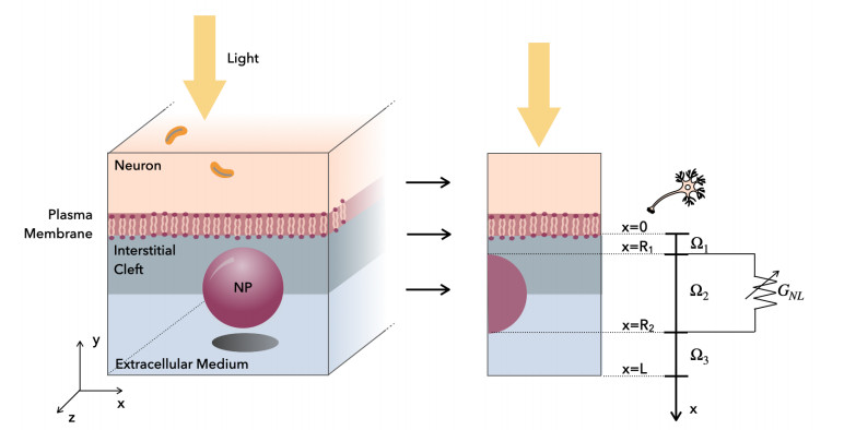
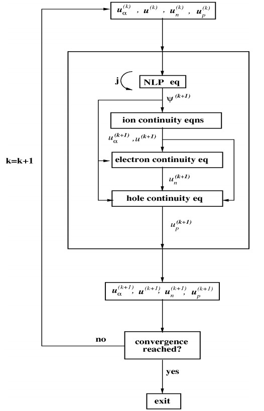
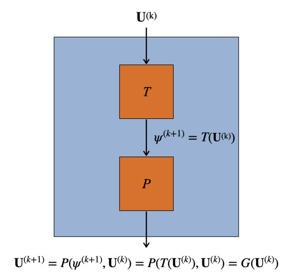
In this article we investigate a mathematical model for a retinal prosthesis made of organic polymer nanoparticles (NP) in the stationary regime. The model consists of a Drift-Diffusion system to describe free charge transport in the NP bulk; a Poisson-Nernst-Planck system to describe ion electrodiffusion in the solution surrounding the NP; and nonlinear transmission conditions at the NP-solution interface. To solve the model we use an iteration procedure for which we prove the existence and briefly comment the uniqueness of a fixed point under suitable smallness assumptions on model parameters. For system discretization we use a stabilized finite element method to prevent unphysical oscillations in the electric potential, carrier number densities and ion molar densities. Model predictions describe the amount of active chemical molecule accumulating at the neuron surface and highlight electrostatic effects induced by the sole presence of the nanoparticle. These results support the use of mathematical modeling as a virtual laboratory for the optimal design of bio-hybrid systems, whose investigation may be impervious due to experimental limits.
- multiscale and multiphysics modeling,
- nonlinear interface coupling,
- ion electrodiffusion,
- drift-diffusion charge transport,
- neuron depolarization,
- functional iterations
Citation: Greta Chiaravalli, Guglielmo Lanzani, Riccardo Sacco, Sandro Salsa. Nanoparticle-based organic polymer retinal prostheses: modeling, solution map and simulation[J]. Mathematics in Engineering, 2023, 5(4): 1-44. doi: 10.3934/mine.2023075

Related Papers:

Abstract

In this article we investigate a mathematical model for a retinal prosthesis made of organic polymer nanoparticles (NP) in the stationary regime. The model consists of a Drift-Diffusion system to describe free charge transport in the NP bulk; a Poisson-Nernst-Planck system to describe ion electrodiffusion in the solution surrounding the NP; and nonlinear transmission conditions at the NP-solution interface. To solve the model we use an iteration procedure for which we prove the existence and briefly comment the uniqueness of a fixed point under suitable smallness assumptions on model parameters. For system discretization we use a stabilized finite element method to prevent unphysical oscillations in the electric potential, carrier number densities and ion molar densities. Model predictions describe the amount of active chemical molecule accumulating at the neuron surface and highlight electrostatic effects induced by the sole presence of the nanoparticle. These results support the use of mathematical modeling as a virtual laboratory for the optimal design of bio-hybrid systems, whose investigation may be impervious due to experimental limits.

References

[1]	E. Arnault, C. Barrau, C. Nanteau, P. Gondouin, K. Bigot, F. Viénot, et al., Phototoxic action spectrum on a retinal pigment epithelium model of age-related macular degeneration exposed to sunlight normalized conditions, PLoS ONE, 8 (2013), e71398. https://doi.org/10.1371/journal.pone.0071398 doi: 10.1371/journal.pone.0071398
[2]	F. Benfenati, G. Lanzani, New technologies for developing second generation retinal prostheses, Lab Anim., 47 (2018), 71–75. https://doi.org/10.1038/s41684-018-0003-1 doi: 10.1038/s41684-018-0003-1
[3]	S. Bellani, D. Fazzi, P. Bruno, E. Giussani, E. V. Canesi, G. Lanzani, et al., Reversible p3ht/oxygen charge transfer complex identification in thin films exposed to direct contact with water, J. Phys. Chem. C, 118 (2014), 6291–6299. https://doi.org/10.1021/jp4119309 doi: 10.1021/jp4119309
[4]	G. Chiaravalli, G. Manfredi, R. Sacco, G. Lanzani, Photoelectrochemistry and drift-diffusion simulations in a polythiophene film interfaced with an electrolyte, ACS Appl. Mater. Interfaces, 13 (2021), 36595–36604. https://doi.org/10.1021/acsami.1c10158 doi: 10.1021/acsami.1c10158
[5]	H. Dember, Über eine photoelektronische kraft in kupferoxydul-kristallen, Phys. Z., 32 (1931), 554.
[6]	S. Francia, D. Shmal, S. Di Marco, G. Chiaravalli, J. F. Maya-Vetencourt, G. Mantero, et al., Light-induced charge generation in polymeric nanoparticles restores vision in advanced-stage retinitis pigmentosa rats, Nat. Commun., 13 (2022), 3677. https://doi.org/10.1038/s41467-022-31368-3 doi: 10.1038/s41467-022-31368-3
[7]	A. García-Layana, F. Cabrera-López, J. García-Arumí, L. Arias-Barquet, J. M. Ruiz-Moreno, Early and intermediate age-related macular degeneration: update and clinical review, Clin. Interv. Aging, 12 (2017), 1579–1587. https://doi.org/10.2147/CIA.S142685 doi: 10.2147/CIA.S142685
[8]	D. Ghezzi, M. R. Antognazza, R. Maccarone, S. Bellani, E. Lanzarini, N. Martino, et al., A polymer optoelectronic interface restores light sensitivity in blind rat retinas, Nature Photon., 7 (2013), 400–406. https://doi.org/10.1038/nphoton.2013.34 doi: 10.1038/nphoton.2013.34
[9]	S. R. Goldman, K. Kalikstein, B. Kramer, Dember‐effect theory, J. Appl. Phys., 49 (1978), 2849–2854. https://doi.org/10.1063/1.325166 doi: 10.1063/1.325166
[10]	H. K. Gummel, A self-consistent iterative scheme for one-dimensional steady state transistor calculations, IEEE Trans. Electron Dev., 11 (1964), 455–465. https://doi.org/10.1109/T-ED.1964.15364 doi: 10.1109/T-ED.1964.15364
[11]	F. G. Holz, S. Schmitz-Valckenberg, M. Fleckenstein, Recent developments in the treatment of age-related macular degeneration, J. Clin. Invest., 124 (2014), 1430–1438. https://doi.org/10.1172/JCI71029 doi: 10.1172/JCI71029
[12]	J. W. Jerome, Analysis of charge transport, Heidelberg: Springer, 1996. https://doi.org/10.1007/978-3-642-79987-7
[13]	J. W. Jerome, Analytical approaches to charge transport in a moving medium, Transport Theory Stat. Phys., 31 (2002), 333–366. https://doi.org/10.1081/TT-120015505 doi: 10.1081/TT-120015505
[14]	J. W. Jerome, R. Sacco, Global weak solutions for an incompressible charged fluid with multi-scale couplings: initial–boundary-value problem, Nonlinear Anal., 71 (2009), e2487–e2497. https://doi.org/10.1016/j.na.2009.05.047 doi: 10.1016/j.na.2009.05.047
[15]	J. Q. Li, T. Welchowski, M. Schmid, M. M. Mauschitz, F. G. Holz, R. P. Finger, Prevalence and incidence of age-related macular degeneration in Europe: a systematic review and meta-analysis, Brit. J. Ophthalmol., 104 (2020), 1077–1084. https://doi.org/0.1136/bjophthalmol-2019-314422
[16]	J. L. Lions, E. Magenes, Non-homogeneous boundary value problems and applications (Vol. 1), Heidelberg: Springer, 1972. https://doi.org/10.1007/978-3-642-65161-8
[17]	R. A. Marcus, On the theory of electron‐transfer reactions. Ⅵ. Unified treatment for homogeneous and electrode reactions, J. Chem. Phys., 43 (1965), 679. https://doi.org/10.1063/1.1696792 doi: 10.1063/1.1696792
[18]	P. A. Markowich, The stationary semiconductor device equations, Vienna: Springer, 1986. https://doi.org/10.1007/978-3-7091-3678-2
[19]	N. L. Mata, R. Vogel, Pharmacologic treatment of atrophic age-related macular degeneration, Curr. Opin. Ophthalmol., 21 (2010), 190–196. https://doi.org/10.1097/ICU.0b013e32833866c8 doi: 10.1097/ICU.0b013e32833866c8
[20]	J. F. Maya-Vetencourt, G. Manfredi, M. Mete, E. Colombo, M. Bramini, S. Di Marco, et al., Subretinally injected semiconducting polymer nanoparticles rescue vision in a rat model of retinal dystrophy, Nat. Nanotechnol., 15 (2020), 698–708. https://doi.org/10.1038/s41565-020-0696-3 doi: 10.1038/s41565-020-0696-3
[21]	K. L. Pennington, M. M. DeAngelis, Epidemiology of age-related macular degeneration (AMD): associations with cardiovascular disease phenotypes and lipid factors, Eye Vision, 3 (2016), 1–20. https://doi.org/10.1186/s40662-016-0063-5 doi: 10.1186/s40662-016-0063-5
[22]	S. Picaud, J.-A. Sahel, Retinal prostheses: clinical results and future challenges, C. R. Biol., 337 (2014). 214–222. https://doi.org/10.1016/j.crvi.2014.01.001 doi: 10.1016/j.crvi.2014.01.001
[23]	I. Rubinstein, Electro-diffusion of ions, SIAM, 1990. https://doi.org/10.1137/1.9781611970814
[24]	R. Sacco, G. Guidoboni, A. G. Mauri, A comprehensive physically based approach to modeling in bioengineering and life sciences, Academic Press, 2019. https://doi.org/10.1016/C2016-0-02357-4
[25]	D. L. Scharfetter, H. K. Gummel, Large-signal analysis of a silicon Read diode oscillator, IEEE Trans. Electron Dev., 16 (1969), 64–77. https://doi.org/10.1109/T-ED.1969.16566 doi: 10.1109/T-ED.1969.16566
[26]	U. Schmidt-Erfurth, T. Hasan, Mechanisms of action of photodynamic therapy with verteporfin for the treatment of age-related macular degeneration, Surv. Ophthalmol., 45 (2000), 195–214. https://doi.org/10.1016/S0039-6257(00)00158-2 doi: 10.1016/S0039-6257(00)00158-2
[27]	M. Schmuck, Analysis of the Navier-Stokes-Nernst-Planck-Poisson system, Math. Mod. Meth. Appl. Sci., 19 (2009), 993–1014. https://doi.org/10.1142/S0218202509003693 doi: 10.1142/S0218202509003693
[28]	W. Shockley, W. T. Read, Statistics of the recombinations of holes and electrons, Phys. Rev., 87 (1952), 835–842. https://doi.org/10.1103/PhysRev.87.835 doi: 10.1103/PhysRev.87.835
[29]	J. W. Slotboom, Computer-aided two-dimensional analysis of bipolar transistors, IEEE Trans. Electron Dev., 20 (1973), 669–679. https://doi.org/10.1109/T-ED.1973.17727 doi: 10.1109/T-ED.1973.17727
[30]	W. Van Roosbroeck, Theory of flow of electrons and holes in germanium and other semiconductors, The Bell System Technical Journal, 29 (1950), 560–607. https://doi.org/10.1002/j.1538-7305.1950.tb03653.x doi: 10.1002/j.1538-7305.1950.tb03653.x
[31]	A. L. Wang, D. K. Knight, T.-T. T. Vu, M. C. Mehta, Retinitis pigmentosa: review of current treatment, International Ophthalmology Clinics, 59 (2019), 263–280. https://doi.org/10.1097/IIO.0000000000000256 doi: 10.1097/IIO.0000000000000256
[32]	J. O. Winter, S. F. Cogan, J. F. Rizzo, Retinal prostheses: current challenges and future outlook, J. Biomat. Sci. Polym. Ed., 18 (2007), 1031–1055. https://doi.org/10.1163/156856207781494403 doi: 10.1163/156856207781494403

Reader Comments

Your name:*

Email:*
© 2023 the Author(s), licensee AIMS Press. This is an open access article distributed under the terms of the Creative Commons Attribution License (http://creativecommons.org/licenses/by/4.0)