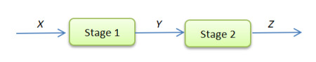
DEA (Data Envelopment Analysis) production games combine DEA theory with cooperation games and assess the benefits to production organizations with single-stage structure. However, in practical production problems, the production organizations are always with network structures. The structure of the production organization not only affects its own benefits, but also relates to the cooperation among organizations. Therefore, it is necessary to study DEA production games with network structures. In this paper, we consider the production organizations with two-stage processes, wherein the organizations are assumed to possess available resources and own technologies. The technology level of each organization is reflected by the observed units based on the network DEA (NDEA) production possibility set. Suppose that the organizations can cooperate through the ways of pooling the initial resources and (or) sharing the technology in each production process. According to the different cooperation styles of each stage in the alliance, seven types of cooperation among organizations are considered. The models of maximizing the revenues of coalitions, namely the NDEA production games, are established corresponding to the seven types, by which the maximal revenue for each coalition can be calculated. We prove that two-stage DEA production games have the super-additive property, and can be expressed as linear programming games. Hence, they are equivalent to the linear production games, and they are totally balanced. Therefore, the proposed cooperative games have a non-empty core, and hence have nucleolus, and the Owen set belongs to the core. In addition, based on the basic conceptions of the nucleolus and the Owen set, the revenue can be allocated among organizations in the alliance. Finally, a numerical example and an empirical application to 17 bank branches of the China Construction Bank in the Anhui Province are presented to illustrate the applicability of the proposed approach, and the relationship between the cooperative manners and the revenue allocation is reflected in analytical results.
Citation: Qianwei Zhang, Zhihua Yang, Binwei Gui. Two-stage network data envelopment analysis production games[J]. AIMS Mathematics, 2024, 9(2): 4925-4961. doi: 10.3934/math.2024240
DEA (Data Envelopment Analysis) production games combine DEA theory with cooperation games and assess the benefits to production organizations with single-stage structure. However, in practical production problems, the production organizations are always with network structures. The structure of the production organization not only affects its own benefits, but also relates to the cooperation among organizations. Therefore, it is necessary to study DEA production games with network structures. In this paper, we consider the production organizations with two-stage processes, wherein the organizations are assumed to possess available resources and own technologies. The technology level of each organization is reflected by the observed units based on the network DEA (NDEA) production possibility set. Suppose that the organizations can cooperate through the ways of pooling the initial resources and (or) sharing the technology in each production process. According to the different cooperation styles of each stage in the alliance, seven types of cooperation among organizations are considered. The models of maximizing the revenues of coalitions, namely the NDEA production games, are established corresponding to the seven types, by which the maximal revenue for each coalition can be calculated. We prove that two-stage DEA production games have the super-additive property, and can be expressed as linear programming games. Hence, they are equivalent to the linear production games, and they are totally balanced. Therefore, the proposed cooperative games have a non-empty core, and hence have nucleolus, and the Owen set belongs to the core. In addition, based on the basic conceptions of the nucleolus and the Owen set, the revenue can be allocated among organizations in the alliance. Finally, a numerical example and an empirical application to 17 bank branches of the China Construction Bank in the Anhui Province are presented to illustrate the applicability of the proposed approach, and the relationship between the cooperative manners and the revenue allocation is reflected in analytical results.

| [1] |
M. Akram, S. M. U. Shah, M. A. Al-Shamiri, S. A. Edalatpanah, Extended DEA method for solving multi-objective transportation problem with Fermatean fuzzy sets, AIMS Math., 8 (2022), 924–961. https://doi.org/10.3934/math.2023045 doi: 10.3934/math.2023045

|
| [2] |
Q. X. An, Y. Wen, J. F. Chu, X. H. Chen, Profit inefficiency decomposition in a serial-structure system with resource sharing, J. Oper. Res. Soc., 70 (2019), 2112–2126. https://doi.org/10.1080/01605682.2018.1510810 doi: 10.1080/01605682.2018.1510810
|
| [3] |
Q. X. An, Y. Wen, T. Ding, Y. L. Li, Resource sharing and payoff allocation in a three-stage system: Integrating network DEA with the Shapley value method, Omega-Internat. J. Man. Sci., 85 (2019), 16–25. https://doi.org/10.1016/j.omega.2018.05.008 doi: 10.1016/j.omega.2018.05.008
|
| [4] |
D. V. Borrero, M. A. Hinojosa, A. M. Marmol, DEA production games and Owen allocations, Eur. J. Oper. Res., 252 (2016), 921–930. https://doi.org/10.1016/j.ejor.2016.01.053 doi: 10.1016/j.ejor.2016.01.053
|
| [5] |
A. Charnes, W. W. Cooper, E. Rhodes, Measuring the efficiency of decision-making units, Eur. J. Oper. Res., 3 (1979), 339–339. https://doi.org/Doi10.1016/0377-2217(79)90229-7 doi: 10.1016/0377-2217(79)90229-7
|
| [6] |
W. D. Cook, L. Liang, J. Zhu, Measuring performance of two-stage network structures by DEA: A review and future perspective, Omega-Internat. J. Man. Sci., 38 (2010), 423–430. https://doi.org/10.1016/j.omega.2009.12.001 doi: 10.1016/j.omega.2009.12.001
|
| [7] | I. Curiel, Cooperative Game Theory and Applications: Cooperative Games Arising From Combinatorial Optimization Problems, Boston: Kluwer Academic Publishers, 1997. |
| [8] |
Q. Z. Dai, Y. J. Li, X. Y. Lei, D. S. Wu, A DEA-based incentive approach for allocating common revenues or fixed costs, Eur. J. Oper. Res., 292 (2021), 675–686. https://doi.org/10.1016/j.ejor.2020.11.006 doi: 10.1016/j.ejor.2020.11.006
|
| [9] |
T. Ding, J. Yang, H. Q. Wu, Y. Wen, C. C. Tan, L. Liang, Research performance evaluation of Chinese university: A non-homogeneous network DEA approach, J. Man. Sci. Eng., 6 (2021), 467–481. https://doi.org/10.1016/j.jmse.2020.10.003 doi: 10.1016/j.jmse.2020.10.003
|
| [10] | R. Fare, S. Grosskopf, Network DEA, Socio-Econ. Plan. Sci., 34 (2000), 35–49. |
| [11] |
F. R. Fernández, M. G. Fiestras-Janeiro, I. Garcia-Jurado, J. Puerto, Competition and cooperation in non-centralized linear production games, Ann. Oper. Res., 137 (2005), 91–100. https://doi.org/10.1007/s10479-005-2247-6 doi: 10.1007/s10479-005-2247-6
|
| [12] |
D. Gong, S. Liu, X. Lu, Modelling the impacts of resource sharing on supply chain efficiency, Internat. J. Simu. Model., 14 (2015), 744–755. https://doi.org/10.2507/Ijsimm14(4)Co20 doi: 10.2507/Ijsimm14(4)Co20
|
| [13] | J. González-Díaz, I. Garcıa-Jurado, M. G. Fiestras-Janeiro, An Introductory Course on Mathematical Game Theory, Graduate Studies in Mathematics, Providence: American Mathematical Society, 2010. |
| [14] |
J. C. Hennet, S. Mahjoub, Toward the fair sharing of profit in a supply network formation, Internat. J. Prod. Econ., 127 (2010), 112–120. https://doi.org/10.1016/j.ijpe.2010.04.047 doi: 10.1016/j.ijpe.2010.04.047
|
| [15] |
M. A. Hinojosa, S. Lozano, A. M. Mármol, DEA production games with fuzzy output prices, Fuzzy Optim. Decis. Mak., 17 (2018), 401–419. https://doi.org/10.1007/s10700-017-9278-8 doi: 10.1007/s10700-017-9278-8
|
| [16] |
G. R. Jahanshahloo, M. Soleimani-damaneh, A. Mostafaee, On the computational complexity of cost efficiency analysis models, Appl. Math. Comput., 188 (2007), 638–640. https://doi.org/10.1016/j.amc.2006.10.030 doi: 10.1016/j.amc.2006.10.030
|
| [17] |
H. H. Jiang, J. Wu, J. F. Chu, H. W. Liu, Better resource utilization: A new DEA bi-objective resource reallocation approach considering environmental efficiency improvement, Comput. Ind. Eng., 144 (2020), 106504. https://doi.org/10.1016/j.cie.2020.106504 doi: 10.1016/j.cie.2020.106504
|
| [18] |
S. Kaffash, R. Azizi, Y. Huang, J. Zhu, A survey of data envelopment analysis applications in the insurance industry 1993–2018, Eur. J. Oper. Res., 284 (2020), 801–813. https://doi.org/10.1016/j.ejor.2019.07.034 doi: 10.1016/j.ejor.2019.07.034
|
| [19] |
C. Kao, Efficiency decomposition for general multi-stage systems in data envelopment analysis, Eur. J. Oper. Res., 232 (2014), 117–124. https://doi.org/10.1016/j.ejor.2013.07.012 doi: 10.1016/j.ejor.2013.07.012
|
| [20] |
C. Kao, Network data envelopment analysis: A review, Eur. J. Oper. Res., 239 (2014), 1–16. https://doi.org/10.1016/j.ejor.2014.02.039 doi: 10.1016/j.ejor.2014.02.039
|
| [21] |
M. Khoveyni, R. Eslami, Two-stage network DEA with shared resources: Illustrating the drawbacks and measuring the overall efficiency, Knowledge-Based Syst., 250 (2022), 108725. https://doi.org/10.1016/j.knosys.2022.108725 doi: 10.1016/j.knosys.2022.108725
|
| [22] |
F. Li, Q. Y. Zhu, Z. Chen, Allocating a fixed cost across the decision making units with two-stage network structures, Omega-Internat. J. Man. Sci., 83 (2019), 139–154. https://doi.org/10.1016/j.omega.2018.02.009 doi: 10.1016/j.omega.2018.02.009
|
| [23] |
F. Li, Q. Y. Zhu, L. Liang, A new data envelopment analysis based approach for fixed cost allocation, Ann. Oper. Res., 274 (2019), 347–372. https://doi.org/10.1007/s10479-018-2819-x doi: 10.1007/s10479-018-2819-x
|
| [24] |
H. T. Li, C. L. Chen, W. D. Cook, J. L. Zhang, J. Zhu, Two-stage network DEA: Who is the leader? Omega-Internat. J. Man. Sci., 74 (2018), 15–19. https://doi.org/10.1016/j.omega.2016.12.009 doi: 10.1016/j.omega.2016.12.009
|
| [25] |
Y. J. Li, L. Lin, Q. Z. Dai, L. D. Zhang, Allocating common costs of multinational companies based on arm's length principle and Nash non-cooperative game, Eur. J. Oper. Res., 283 (2020), 1002–1010. https://doi.org/10.1016/j.ejor.2019.11.049 doi: 10.1016/j.ejor.2019.11.049
|
| [26] |
L. Liang, W. D. Cook, J. Zhu, DEA models for two-stage processes: Game approach and efficiency decomposition, Naval Res. Logist., 55 (2008), 643–653. https://doi.org/10.1002/nav.20308 doi: 10.1002/nav.20308
|
| [27] |
S. Lozano, Information sharing in DEA: A cooperative game theory approach, Eur. J. Oper. Res., 222 (2012), 558–565. https://doi.org/10.1016/j.ejor.2012.05.014 doi: 10.1016/j.ejor.2012.05.014
|
| [28] |
S. Lozano, DEA production games, Eur. J. Oper. Res., 231 (2013), 405–413. https://doi.org/10.1016/j.ejor.2013.06.004 doi: 10.1016/j.ejor.2013.06.004
|
| [29] |
S. Lozano, M. A. Hinojosa, A. M. Marmol, Set-valued DEA production games, Omega-Internat. J. Man. Sci., 52 (2015), 92–100. https://doi.org/10.1016/j.omega.2014.10.002 doi: 10.1016/j.omega.2014.10.002
|
| [30] |
J. F. Ma, A two-stage DEA model considering shared inputs and free intermediate measures, Expert Syst. Appl., 42 (2015), 4339–4347. https://doi.org/10.1016/j.eswa.2015.01.040 doi: 10.1016/j.eswa.2015.01.040
|
| [31] |
J. F. Ma, T. M. D. Zhao, Operating efficiency assessment of commercial banks with cooperative-stackelberg hybrid two-stage DEA, RAIRO-Oper. Res., 55 (2021), 3197–3215. https://doi.org/10.1051/ro/2021152 doi: 10.1051/ro/2021152
|
| [32] |
G. Owen, On the core of linear production games, Math. Program., 9 (1975), 358–370. https://doi.org/10.1007/BF01681356 doi: 10.1007/BF01681356
|
| [33] | H. Peters, Game Theory: A Multi-Leveled Approach, Berlin-Heidelberg: Springer, 2008. |
| [34] |
D. Schmeidler, The nucleolus of a characteristic function game, SIAM J. Appl. Math., 17 (1969), 1163–1170. https://doi.org/10.1137/0117107 doi: 10.1137/0117107
|
| [35] | L. S. Shapley, On balanced sets and cores, Naval Res. Logist. Quart., 14 (1965), 453–460. |
| [36] |
S. Soofizadeh, R. Fallahnejad, Evaluation of groups using cooperative game with fuzzy data envelopment analysis, AIMS Math., 8 (2023), 8661–8679. https://doi.org/10.3934/math.2023435 doi: 10.3934/math.2023435
|
| [37] |
J. Timmer, P. Borm, J. Suijs, Linear transformation of products: Games and economies, J. Optim. Theo. Appl., 105 (2000), 677–706. https://doi.org/10.1023/A:1004601509292 doi: 10.1023/A:1004601509292
|
| [38] |
J. R. G. van Gellekom, J. A. M. Potters, J. H. Reijnierse, M. C. Engel, Characterization of the Owen set of linear production processes, Games Econ. Behav., 32 (2000), 139–156. https://doi.org/10.1006/game.1999.0758 doi: 10.1006/game.1999.0758
|
| [39] |
Y. Wen, Q. X. An, J. H. Hu, X. H. Chen, DEA game for internal cooperation between an upper-level process and multiple lower-level processes, J. Oper. Res. Soc., 73 (2022), 1949–1960. https://doi.org/10.1080/01605682.2021.1967212 doi: 10.1080/01605682.2021.1967212
|
| [40] |
J. Wu, Q. Y. Zhu, W. D. Cooke, J. Zhu, Best cooperative partner selection and input resource reallocation using DEA, J. Oper. Res. Soc., 67 (2016), 1221–1237. https://doi.org/10.1057/jors.2016.26 doi: 10.1057/jors.2016.26
|
| [41] |
F. Yang, Y. Sun, D. W. Wang, S. Ang, Network data envelopment analysis with two-level maximin strategy, RAIRO-Oper. Res., 56 (2022), 2543–2556. https://doi.org/10.1051/ro/2022090 doi: 10.1051/ro/2022090
|
| [42] |
F. Yang, D. X. Wu, L. Liang, G. B. Bi, D. D. Wu, Supply chain DEA: production possibility set and performance evaluation model, Ann. Oper. Res., 185 (2011), 195–211. https://doi.org/10.1007/s10479-008-0511-2 doi: 10.1007/s10479-008-0511-2
|
| [43] |
Q. W. Zhang, Z. H. Yang, Returns to scale of two-stage production process, Comput. Ind. Eng., 90 (2015), 259–268. https://doi.org/10.1016/j.cie.2015.09.009 doi: 10.1016/j.cie.2015.09.009
|
Figures(2) / Tables(14)

Qianwei Zhang, Zhihua Yang, Binwei Gui. Two-stage network data envelopment analysis production games[J]. AIMS Mathematics, 2024, 9(2): 4925-4961. doi: 10.3934/math.2024240


 DownLoad: