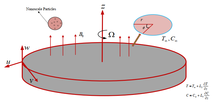
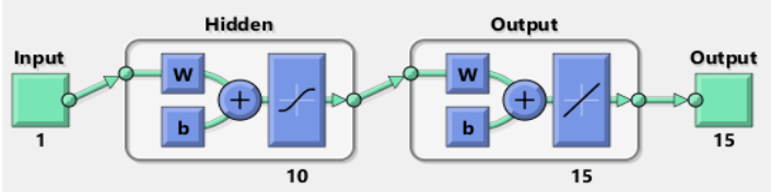
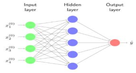
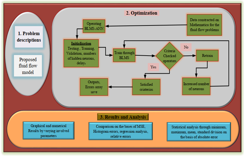
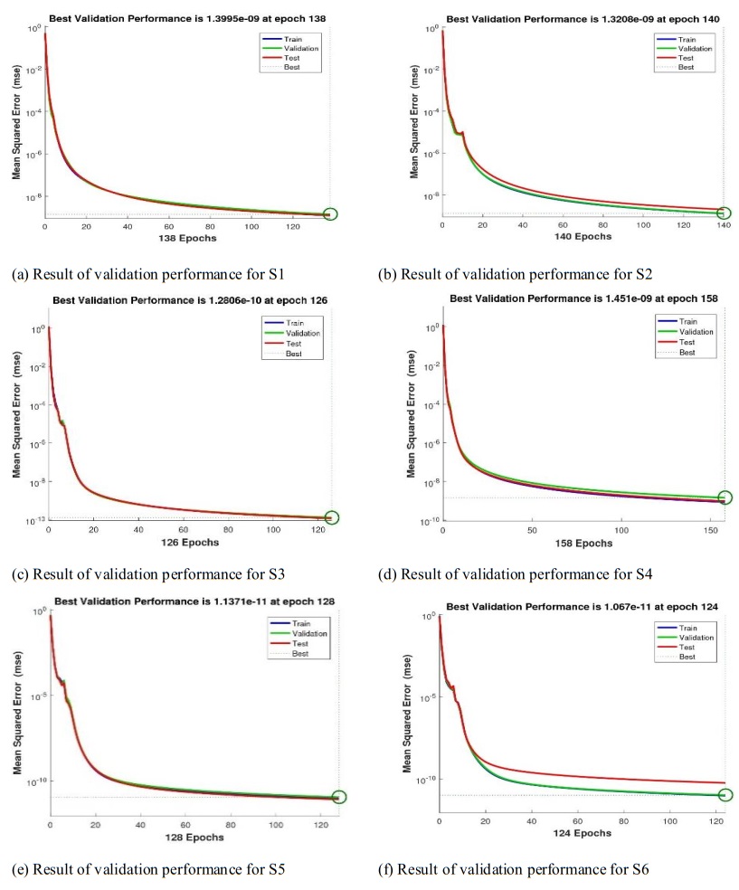
In this paper, the neural network domain with the backpropagation Levenberg-Marquardt scheme (NNB-LMS) is novel with a convergent stability and generates a numerical solution of the impact of the magnetohydrodynamic (MHD) nanofluid flow over a rotating disk (MHD-NRD) with heat generation/absorption and slip effects. The similarity variation in the MHD flow of a viscous liquid through a rotating disk is explained by transforming the original non-linear partial differential equations (PDEs) to an equivalent non-linear ordinary differential equation (ODEs). Varying the velocity slip parameter, Hartman number, thermal slip parameter, heat generation/absorption parameter, and concentration slip parameter, generates a Prandtl number using the Runge-Kutta 4th order method (RK4) numerical technique, which is a dataset for the suggested (NNB-LMS) for numerous MHD-NRD scenarios. The validity of the data is tested, and the data is processed and properly tabulated to test the exactness of the suggested model. The recommended model was compared for verification, and the estimation solutions for particular instances were assessed using the NNB-LMS training, testing, and validation procedures. A regression analysis, a mean squared error (MSE) assessment, and a histogram analysis were used to further evaluate the proposed NNB-LMS. The NNB-LMS technique has various applications such as disease diagnosis, robotic control systems, ecosystem evaluation, etc. Some statistical data such as the gradient, performance, and epoch of the model were analyzed. This recommended method differs from the reference and suggested results, and has an accuracy rating ranging from $ {10}^{-09} $to $ {10}^{-12} $.
Citation: Yousef Jawarneh, Humaira Yasmin, Wajid Ullah Jan, Ajed Akbar, M. Mossa Al-Sawalha. A neural networks technique for analysis of MHD nano-fluid flow over a rotating disk with heat generation/absorption[J]. AIMS Mathematics, 2024, 9(11): 32272-32298. doi: 10.3934/math.20241549
In this paper, the neural network domain with the backpropagation Levenberg-Marquardt scheme (NNB-LMS) is novel with a convergent stability and generates a numerical solution of the impact of the magnetohydrodynamic (MHD) nanofluid flow over a rotating disk (MHD-NRD) with heat generation/absorption and slip effects. The similarity variation in the MHD flow of a viscous liquid through a rotating disk is explained by transforming the original non-linear partial differential equations (PDEs) to an equivalent non-linear ordinary differential equation (ODEs). Varying the velocity slip parameter, Hartman number, thermal slip parameter, heat generation/absorption parameter, and concentration slip parameter, generates a Prandtl number using the Runge-Kutta 4th order method (RK4) numerical technique, which is a dataset for the suggested (NNB-LMS) for numerous MHD-NRD scenarios. The validity of the data is tested, and the data is processed and properly tabulated to test the exactness of the suggested model. The recommended model was compared for verification, and the estimation solutions for particular instances were assessed using the NNB-LMS training, testing, and validation procedures. A regression analysis, a mean squared error (MSE) assessment, and a histogram analysis were used to further evaluate the proposed NNB-LMS. The NNB-LMS technique has various applications such as disease diagnosis, robotic control systems, ecosystem evaluation, etc. Some statistical data such as the gradient, performance, and epoch of the model were analyzed. This recommended method differs from the reference and suggested results, and has an accuracy rating ranging from $ {10}^{-09} $to $ {10}^{-12} $.

| [1] |
B. M. Wilamowski, H. Yu, Improved computation for Levenberg-Marquardt training, IEEE Trans. Neur. Net., 21 (2010), 930–937. https://doi.org/10.1109/TNN.2010.2045657 doi: 10.1109/TNN.2010.2045657

|
| [2] |
D. B. Parker, A comparison of algorithms for neuron‐like cells, AIP Conf. Proc., 151 (1986), 327–332. https://doi.org/10.1063/1.36233 doi: 10.1063/1.36233
|
| [3] |
A. Akbar, H. Ullah, M. A. Z. Raja, K. S. Nisar, S. Islam, M. Shoaib, 2022. A design of neural networks to study MHD and heat transfer in two phase model of nano-fluid flow in the presence of thermal radiation, Waves Random Complex Media, 2022, 1–24. https://doi.org/10.1080/17455030.2022.2152905 doi: 10.1080/17455030.2022.2152905
|
| [4] |
M. Shoaib, M. A. Z. Raja, M. T. Sabir, S. Islam, Z. Shah, P. Kumam, et al., Numerical investigation for rotating flow of MHD hybrid nanofluid with thermal radiation over a stretching sheet, Sci. Rep., 10 (2020), 18533. https://doi.org/10.1038/s41598-020-75254-8 doi: 10.1038/s41598-020-75254-8
|
| [5] |
R. A. Khan, H. Ullah, M. A. Z. Raja, M. A. R. Khan, S. Islam, M. Shoaib, Heat transfer between two porous parallel plates of steady nano fludis with Brownian and Thermophoretic effects: a new stochastic numerical approach, Int. Commun. Heat Mass Transfer, 126 (2021), 105436. https://doi.org/10.1016/j.icheatmasstransfer.2021.105436 doi: 10.1016/j.icheatmasstransfer.2021.105436
|
| [6] |
Z. Sabir, M. A. Z. Raja, J. L. Guirao, M. Shoaib, Integrated intelligent computing with neuro-swarming solver for multi-singular fourth-order nonlinear Emden-Fowler equation, Comp. Appl. Math., 39 (2020), 307. https://doi.org/10.1007/s40314-020-01330-4 doi: 10.1007/s40314-020-01330-4
|
| [7] |
H. Yasmin, L. A. AL-Essa, A. M. Mahnashi, W. Hamali, A. Saeed, A magnetohydrodynamic flow of a water-based hybrid nanofluid past a convectively heated rotating disk surface: a passive control of nanoparticles, Rev. Adv. Mater. Sci., 63 (2024), 20240054. https://doi.org/10.1515/rams-2024-0054 doi: 10.1515/rams-2024-0054
|
| [8] |
M. M. Al-Sawalha, H. Yasmin, S. Muhammad, Y. Khan, R. Shah, Optimal power management of a stand-alone hybrid energy management system: hydro-photovoltaic-fuel cell, Ain Shams Eng. J., 2024, 103089. https://doi.org/10.1016/j.asej.2024.103089 doi: 10.1016/j.asej.2024.103089
|
| [9] | K. B. Pavlov, Magnetohydrodynamic flow of an incompressible viscous fluid caused by deformation of a plane surface, Magn. Gidrodin., 4 (1974), 146–147. |
| [10] |
A. A. Aldhafeeri, H. Yasmin, A numerical analysis of the rotational flow of a hybrid nanofluid past a unidirectional extending surface with velocity and thermal slip conditions, Rev. Adv. Mater. Sci., 63 (2024), 20240052. https://doi.org/10.1515/rams-2024-0052 doi: 10.1515/rams-2024-0052
|
| [11] | A. Chakrabarti, A. S. Gupta, Hydromagnetic flow and heat transfer over a stretching sheet, Q. Appl. Math., 37 (1979), 73–78. |
| [12] |
M. R. Khan, S. Mao, Numerical solution of magnetohydrodynamics radiative flow of Oldroyd-B nanofluid toward a porous stretched surface containing gyrotactic microorganisms, ZAMM‐J. Appl. Math. Mech./Z. Angew. Math. Mech., 102 (2022), e202100388. https://doi.org/10.1002/zamm.202100388 doi: 10.1002/zamm.202100388
|
| [13] |
H. Yasmin, Numerical investigation of heat and mass transfer study on MHD rotatory hybrid nanofluid flow over a stretching sheet with gyrotactic microorganisms, Ain Shams Eng. J., 15 (2024), 102918. https://doi.org/10.1016/j.asej.2024.102918 doi: 10.1016/j.asej.2024.102918
|
| [14] |
S. Heysiattalab, A. Malvandi, D. D. Ganji, Anisotropic behavior of magnetic nanofluids (MNFs) at filmwise condensation over a vertical plate in presence of a uniform variable-directional magnetic field, J. Mol. Liq., 219 (2016), 875–882. https://doi.org/10.1016/j.molliq.2016.04.004 doi: 10.1016/j.molliq.2016.04.004
|
| [15] |
H. Yasmin, Analytical investigation of convective phenomena with nonlinearity characteristics in nanostratified liquid film above an inclined extended sheet, Nanotechnol. Rev., 13 (2024), 20240064. https://doi.org/10.1515/ntrev-2024-0064 doi: 10.1515/ntrev-2024-0064
|
| [16] |
T. Hayat, A. Aziz, T. Muhammad, A. Alsaedi, On magnetohydrodynamic three-dimensional flow of nanofluid over a convectively heated nonlinear stretching surface, Int. J. Heat Mass Transfer, 100 (2016), 566–572. https://doi.org/10.1016/j.ijheatmasstransfer.2016.04.113 doi: 10.1016/j.ijheatmasstransfer.2016.04.113
|
| [17] |
T. Hayat, M. Waqas, M. I. Khan, A. Alsaedi, Analysis of thixotropic nanomaterial in a doubly stratified medium considering magnetic field effects, Int. J. Heat Mass Transfer, 102 (2016), 1123–1129. https://doi.org/10.1016/j.ijheatmasstransfer.2016.06.090 doi: 10.1016/j.ijheatmasstransfer.2016.06.090
|
| [18] |
M. R. Khan, S. Mao, W. Deebani, A. M. A. Elsiddieg, Numerical analysis of heat transfer and friction drag relating to the effect of Joule heating, viscous dissipation and heat generation/absorption in aligned MHD slip flow of a nanofluid, Int. Commun. Heat Mass Transfer, 131 (2022), 105843. https://doi.org/10.1016/j.icheatmasstransfer.2021.105843 doi: 10.1016/j.icheatmasstransfer.2021.105843
|
| [19] |
A. Malvandi, A. Ghasemi, D. D. Ganji, Thermal performance analysis of hydromagnetic Al2O3-water nanofluid flows inside a concentric microannulus considering nanoparticle migration and asymmetric heating, Int. J. Thermal Sci., 109 (2016), 10–22. https://doi.org/10.1016/j.ijthermalsci.2016.05.023 doi: 10.1016/j.ijthermalsci.2016.05.023
|
| [20] |
A. A. Aldhafeeri, H. Yasmin, Thermal analysis of the water-based micropolar hybrid nanofluid flow comprising diamond and copper nanomaterials past an extending surface, Case Stud. Thermal Eng., 59 (2024), 104466. https://doi.org/10.1016/j.csite.2024.104466 doi: 10.1016/j.csite.2024.104466
|
| [21] |
T. Hayat, T. Muhammad, S. A. Shehzad, A. Alsaedi, An analytical solution for magnetohydrodynamic Oldroyd-B nanofluid flow induced by a stretching sheet with heat generation/absorption, Int. J. Thermal Sci., 111 (2017), 274–288. https://doi.org/10.1016/j.ijthermalsci.2016.08.009 doi: 10.1016/j.ijthermalsci.2016.08.009
|
| [22] | W. Yu, D. M. France, S. U. S. Choi, J. L. Routbort, Review and assessment of nanofluid technology for transportation and other applications, Argonne National Lab. (ANL), Argonne, IL (United States), 2007. https://doi.org/10.2172/919327 |
| [23] |
H. Yasmin, L. A. Al-Essa, R. Bossly, H. Alrabaiah, S. A. Lone, A. Saeed, A homotopic analysis of the blood-based bioconvection Carreau-Yasuda hybrid nanofluid flow over a stretching sheet with convective conditions, Nanotechnol. Rev., 13 (2024), 20240031. https://doi.org/10.1515/ntrev-2024-0031 doi: 10.1515/ntrev-2024-0031
|
| [24] |
H. Yasmin, L. A. AL-Essa, R. Bossly, H. Alrabaiah, S. A. Lone, A. Saeed, A numerical investigation of the magnetized water-based hybrid nanofluid flow over an extending sheet with a convective condition: active and passive controls of nanoparticles, Nanotechnol. Rev., 13 (2024), 20240035. https://doi.org/10.1515/ntrev-2024-0035 doi: 10.1515/ntrev-2024-0035
|
| [25] | S. U. S. Choi, J. A. Eastman, Enhancing thermal conductivity of fluids with nanoparticles, Argonne National Lab. (ANL), Argonne, IL (United States), 1995. |
| [26] |
M. R. Khan, V. Puneeth, M. K. Alaoui, R. Alroobaea, M. M. M. Abdou, Heat transfer in a dissipative nanofluid passing by a convective stretching/shrinking cylinder near the stagnation point, ZAMM-J. Appl. Math. Mech./Z. Angew. Math. Mech., 104 (2024), e202300733. https://doi.org/10.1002/zamm.202300733 doi: 10.1002/zamm.202300733
|
| [27] |
L. Ali, Y. J. Wu, B. Ali, S. Abdal, S. Hussain, The crucial features of aggregation in TiO2-water nanofluid aligned of chemically comprising microorganisms: a FEM approach, Comput. Math. Appl., 123 (2022), 241–251. https://doi.org/10.1016/j.camwa.2022.08.028 doi: 10.1016/j.camwa.2022.08.028
|
| [28] |
A. Raza, A. Ghaffari, S. U. Khan, A. U. Haq, M. I. Khan, M. R. Khan, Non-singular fractional computations for the radiative heat and mass transfer phenomenon subject to mixed convection and slip boundary effects, Chaos Soliton. Fract., 155 (2022), 111708. https://doi.org/10.1016/j.chaos.2021.111708 doi: 10.1016/j.chaos.2021.111708
|
| [29] |
M. Sheikholeslami, T. Hayat, A. Alsaedi, MHD free convection of Al2O3-water nanofluid considering thermal radiation: a numerical study, Int. J. Heat Mass Transfer, 96 (2016), 513–524. https://doi.org/10.1016/j.ijheatmasstransfer.2016.01.059 doi: 10.1016/j.ijheatmasstransfer.2016.01.059
|
| [30] |
A. M. Alqahtani, M. R. Khan, N. Akkurt, V. Puneeth, A. Alhowaity, H. Hamam, Thermal analysis of a radiative nanofluid over a stretching/shrinking cylinder with viscous dissipation, Chem. Phys. Lett., 808 (2022), 140133. https://doi.org/10.1016/j.cplett.2022.140133 doi: 10.1016/j.cplett.2022.140133
|
| [31] |
W. U. Jan, M. Farooq, R. A. Shah, A. Khan, M. S. Zobaer, R. Jan, Flow dynamics of the homogeneous and heterogeneous reactions with an internal heat generation and thermal radiation between two squeezing plates, Mathematics, 9 (2021), 2309. https://doi.org/10.3390/math9182309 doi: 10.3390/math9182309
|
| [32] |
L. Ali, P. Kumar, H. Poonia, S. Areekara, R. Apsari, The significant role of Darcy-Forchheimer and thermal radiation on Casson fluid flow subject to stretching surface: a case study of dusty fluid, Mod. Phys. Lett. B, 38 (2024), 2350215. https://doi.org/10.1142/S0217984923502159 doi: 10.1142/S0217984923502159
|
| [33] |
M. M. Bhatti, M. M. Rashidi, Numerical simulation of entropy generation on MHD nanofluid towards a stagnation point flow over a stretching surface, Int. J. Appl. Comput. Math., 3 (2017), 2275–2289. https://doi.org/10.1007/s40819-016-0193-4 doi: 10.1007/s40819-016-0193-4
|
| [34] |
W. Ibrahim, B. Shankar, M. M. Nandeppanavar, MHD stagnation point flow and heat transfer due to nanofluid towards a stretching sheet, Int. J. Heat Mass Transfer, 56 (2013), 1–9. https://doi.org/10.1016/j.ijheatmasstransfer.2012.08.034 doi: 10.1016/j.ijheatmasstransfer.2012.08.034
|
| [35] |
L. Ali, P. Kumar, Z. Iqbal, S. E. Alhazmi, S. Areekara, M. M. Alqarni, et al., The optimization of heat transfer in thermally convective micropolar-based nanofluid flow by the influence of nanoparticle's diameter and nanolayer via stretching sheet: sensitivity analysis approach, J. Non-Equil. Thermody., 48 (2023), 313–330. https://doi.org/10.1515/jnet-2022-0064 doi: 10.1515/jnet-2022-0064
|
| [36] |
L. Ahmad, M. Irfan, S. Javed, M. I. Khan, M. R. Khan, U. M. Niazi, et al., Influential study of novel microorganism and nanoparticles during heat and mass transport in Homann flow of visco-elastic materials, Int. Commun. Heat Mass Transfer, 131 (2022), 105871. https://doi.org/10.1016/j.icheatmasstransfer.2021.105871 doi: 10.1016/j.icheatmasstransfer.2021.105871
|
| [37] |
L. Ali, B. Ali, M. B. Ghori, Melting effect on Cattaneo-Christov and thermal radiation features for aligned MHD nanofluid flow comprising microorganisms to leading edge: FEM approach, Comput. Math. Appl., 109 (2022), 260–269. https://doi.org/10.1016/j.camwa.2022.01.009 doi: 10.1016/j.camwa.2022.01.009
|
| [38] |
S. Nadeem, S. Ahmad, N. Muhammad, Computational study of Falkner-Skan problem for a static and moving wedge, Sensors Actuat. B: Chem., 263 (2018), 69–76. https://doi.org/10.1016/j.snb.2018.02.039 doi: 10.1016/j.snb.2018.02.039
|
| [39] |
L. Ali, R. Apsari, A. Abbas, P. Tak, Entropy generation on the dynamics of volume fraction of nano-particles and coriolis force impacts on mixed convective nanofluid flow with significant magnetic effect, Numer. Heat Transfer, Part A, 2024, 1–16. https://doi.org/10.1080/10407782.2024.2360652 doi: 10.1080/10407782.2024.2360652
|
| [40] | Z. Hu, W. Lu, M. D. Thouless, Slip and wear at a corner with Coulomb friction and an interfacial strength, Wear, 338-339 (2015), 242–251. https://doi.org/10.1016/j.wear.2015.06.010 |
| [41] |
Z. Hu, W. Lu, M. D. Thouless, J. R. Barber, Effect of plastic deformation on the evolution of wear and local stress fields in fretting, Int. J. Solids Struct., 82 (2016), 1–8. https://doi.org/10.1016/j.ijsolstr.2015.12.031 doi: 10.1016/j.ijsolstr.2015.12.031
|
| [42] |
H. Wang, Z. Hu, W. Lu, M. D. Thouless, The effect of coupled wear and creep during grid-to-rod fretting, Nucl. Eng. Des., 318 (2017), 163–173. https://doi.org/10.1016/j.nucengdes.2017.04.018 doi: 10.1016/j.nucengdes.2017.04.018
|
| [43] | T. Von Karman, Uberlaminare und turbulente Reibung, Z. Angew. Math Mech., 1 (1921), 233–252. |
| [44] |
W. G. Cochran, The flow due to a rotating disk, Math. Proc. Cambridge Philos. Soc., 30 (1934), 365–375. https://doi.org/10.1017/S0305004100012561 doi: 10.1017/S0305004100012561
|
| [45] |
J. A. D. Ackroyd, On the steady flow produced by a rotating disk with either surface suction or injection, J. Eng. Math., 12 (1978), 207–220. https://doi.org/10.1007/BF00036459 doi: 10.1007/BF00036459
|
| [46] |
K. Millsaps, K. Pohlhausen, Heat transfer by laminar flow from a rotating plate, J. Aeronaut. Sci., 19 (1952), 120–126. https://doi.org/10.2514/8.2175 doi: 10.2514/8.2175
|
| [47] |
M. Miklavčič, C. Y. Wang, The flow due to a rough rotating disk, Z. Angew. Math. Phys., 55 (2004), 235–246. https://doi.org/10.1007/s00033-003-2096-6 doi: 10.1007/s00033-003-2096-6
|
| [48] |
R. Alizadeh, N. Karimi, R. Arjmandzadeh, A. Mehdizadeh, Mixed convection and thermodynamic irreversibilities in MHD nanofluid stagnation-point flows over a cylinder embedded in porous media, J. Therm. Anal. Calorim., 135 (2019), 489–506. https://doi.org/10.1007/s10973-018-7071-8 doi: 10.1007/s10973-018-7071-8
|
| [49] |
Z. Shah, H. Babazadeh, P. Kumam, A. Shafee, P. Thounthong, Numerical simulation of magnetohydrodynamic nanofluids under the influence of shape factor and thermal transport in a porous media using CVFEM, Front. Phys., 7 (2019), 164. https://doi.org/10.3389/fphy.2019.00164 doi: 10.3389/fphy.2019.00164
|
| [50] |
H. A. Attia, Steady flow over a rotating disk in porous medium with heat transfer, Nonlinear Anal., 14 (2009), 21–26. https://doi.org/10.15388/NA.2009.14.1.14527 doi: 10.15388/NA.2009.14.1.14527
|
| [51] |
M. Turkyilmazoglu, P. Senel, Heat and mass transfer of the flow due to a rotating rough and porous disk, Int. J. Thermal Sci., 63 (2013), 146–158. https://doi.org/10.1016/j.ijthermalsci.2012.07.013 doi: 10.1016/j.ijthermalsci.2012.07.013
|
| [52] |
Z. Shah, A. Dawar, I. Khan, S. Islam, D. L. C. Ching, A. Z. Khan, Cattaneo-Christov model for electrical magnetite micropoler Casson ferrofluid over a stretching/shrinking sheet using effective thermal conductivity model, Case Stud. Therm. Eng., 13 (2019), 100352. https://doi.org/10.1016/j.csite.2018.11.003 doi: 10.1016/j.csite.2018.11.003
|
| [53] |
M. Mustafa, J. A. Khan, T. Hayat, A. Alsaedi, On Bö dewadt flow and heat transfer of nanofluids over a stretching stationary disk, J. Mol. Liq., 211 (2015), 119–125. https://doi.org/10.1016/j.molliq.2015.06.065 doi: 10.1016/j.molliq.2015.06.065
|
| [54] |
M. M. Rashidi, N. Kavyani, S. Abelman, Investigation of entropy generation in MHD and slip flow over a rotating porous disk with variable properties, Int. J. Heat Mass Transfer, 70 (2014), 892–917. https://doi.org/10.1016/j.ijheatmasstransfer.2013.11.058 doi: 10.1016/j.ijheatmasstransfer.2013.11.058
|
| [55] |
T. Hayat, T. Muhammad, S. A. Shehzad, A. Alsaedi, On magnetohydrodynamic flow of nanofluid due to a rotating disk with slip effect: a numerical study, Comput. Methods Appl. Mech. Eng., 315 (2017), 467–477. https://doi.org/10.1016/j.cma.2016.11.002 doi: 10.1016/j.cma.2016.11.002
|
| [56] |
T. Hayat, F. Haider, T. Muhammad, A. Alsaedi, On Darcy-Forchheimer flow of carbon nanotubes due to a rotating disk, Int. J. Heat Mass Transfer, 112 (2017), 248–254. https://doi.org/10.1016/j.ijheatmasstransfer.2017.04.123 doi: 10.1016/j.ijheatmasstransfer.2017.04.123
|
| [57] |
H. Waqas, S. U. Khan, M. Hassan, M. M. Bhatti, M. Imran, Analysis on the bioconvection flow of modified second-grade nanofluid containing gyrotactic microorganisms and nanoparticles, J. Mol. Liq., 291 (2019), 111231. https://doi.org/10.1016/j.molliq.2019.111231 doi: 10.1016/j.molliq.2019.111231
|
| [58] |
I. Siddique, M. Nadeem, R. Ali, F. Jarad, Bioconvection of MHD second-grade fluid conveying nanoparticles over an exponentially stretching sheet: a biofuel applications, Arab. J. Sci. Eng., 48 (2023), 3367–3380. https://doi.org/10.1007/s13369-022-07129-1 doi: 10.1007/s13369-022-07129-1
|
| [59] |
A. Shafiq, G. Rasool, C. M. Khalique, S. Aslam, Second grade bioconvective nanofluid flow with buoyancy effect and chemical reaction, Symmetry, 12 (2020), 621. https://doi.org/10.3390/sym12040621 doi: 10.3390/sym12040621
|
| [60] |
S. Zuhra, N. S. Khan, Z. Shah, S. Islam, E. Bonyah, Simulation of bioconvection in the suspension of second grade nanofluid containing nanoparticles and gyrotactic microorganisms, Aip Adv., 8 (2018), 105210. https://doi.org/10.1063/1.5054679 doi: 10.1063/1.5054679
|
| [61] |
S. Abbas, S. F. F. Gilani, M. Nazar, M. Fatima, M. Ahmad, Z. U. Nisa, Bio-convection flow of fractionalized second grade fluid through a vertical channel with Fourier's and Fick's laws, Mod. Phys. Lett. B, 37 (2023), 2350069. https://doi.org/10.1142/S0217984923500690 doi: 10.1142/S0217984923500690
|
| [62] |
T. Hayat, Inayatullah, K. Muhammad, A. Alsaedi, Heat transfer analysis in bio-convection second grade nanofluid with Cattaneo-Christov heat flux model, Proc. Inst. Mech. Eng., Part E, 237 (2023), 1117–1124. https://doi.org/10.1177/09544089221097684 doi: 10.1177/09544089221097684
|
| [63] |
N. M. Sarif, M. Z. Salleh, R. Nazar, Numerical solution of flow and heat transfer over a stretching sheet with Newtonian heating using the Keller box method, Procedia Eng., 53 (2013), 542–554. https://doi.org/10.1016/j.proeng.2013.02.070 doi: 10.1016/j.proeng.2013.02.070
|
| [64] |
S. Liao, On the homotopy analysis method for nonlinear problems, Appl. Math. Comput., 147 (2004), 499–513. https://doi.org/10.1016/S0096-3003(02)00790-7 doi: 10.1016/S0096-3003(02)00790-7
|
| [65] |
J. Wang, X. Ye, A weak Galerkin finite element method for second-order elliptic problems, J. Comput. Appl. Math., 241 (2013), 103–115. https://doi.org/10.1016/j.cam.2012.10.003 doi: 10.1016/j.cam.2012.10.003
|
| [66] |
S. S. Motsa, P. G. Dlamini, M. Khumalo, Spectral relaxation method and spectral quasilinearization method for solving unsteady boundary layer flow problems, Adv. Math. Phys., 2014 (2014), 341964. https://doi.org/10.1155/2014/341964 doi: 10.1155/2014/341964
|
| [67] |
T. Hayat, T. Muhammad, A. Alsaedi, M. S. Alhuthali, Magnetohydrodynamic three-dimensional flow of viscoelastic nanofluid in the presence of nonlinear thermal radiation, J. Magn. Magn. Mater., 385 (2015), 222–229. https://doi.org/10.1016/j.jmmm.2015.02.046 doi: 10.1016/j.jmmm.2015.02.046
|
Figures(11) / Tables(2)

Yousef Jawarneh, Humaira Yasmin, Wajid Ullah Jan, Ajed Akbar, M. Mossa Al-Sawalha. A neural networks technique for analysis of MHD nano-fluid flow over a rotating disk with heat generation/absorption[J]. AIMS Mathematics, 2024, 9(11): 32272-32298. doi: 10.3934/math.20241549


 DownLoad: