Identifying the most optimal wearable health technology devices for hospitals is a crucial step in emergency decision-making. The multi-attribute group decision-making method is a widely used and practical approach for selecting wearable health technology devices. However, because of the various factors that must be considered when selecting devices in emergencies, decision-makers often struggle to create a comprehensive assessment method. This study introduced a novel decision-making method that took into account various factors of decision-makers and has the potential to be applied in various other areas of research. First, we introduced a list of aggregation operators based on Pythagorean hesitant fuzzy rough sets, and a detailed description of the desired characteristics of the operators under investigation were provided. The proposed operators were validated by a newly defined score and accuracy function. Second, this paper used the proposed approach to demonstrate the Pythagorean hesitant fuzzy rough technique for order of preference by similarity to ideal solution (TOPSIS) model for multiple attribute decision-making and its stepwise algorithm. We developed a numerical example based on suggested operators for the evaluation framework to tackle the multiple-attribute decision-making problems while evaluating the performance of wearable health technology devices. In the end, the sensitivity analysis has confirmed the performance and reliability of the proposed framework. The findings indicated that the models being examined demonstrated greater reliability and efficacy compared to existing methodologies.
Citation: Attaullah, Sultan Alyobi, Mohammed Alharthi, Yasser Alrashedi. Pythagorean hesitant fuzzy rough multi-attribute decision-making method with application to wearable health technology devices[J]. AIMS Mathematics, 2024, 9(10): 27167-27204. doi: 10.3934/math.20241321
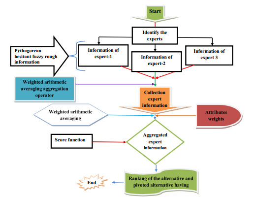
Identifying the most optimal wearable health technology devices for hospitals is a crucial step in emergency decision-making. The multi-attribute group decision-making method is a widely used and practical approach for selecting wearable health technology devices. However, because of the various factors that must be considered when selecting devices in emergencies, decision-makers often struggle to create a comprehensive assessment method. This study introduced a novel decision-making method that took into account various factors of decision-makers and has the potential to be applied in various other areas of research. First, we introduced a list of aggregation operators based on Pythagorean hesitant fuzzy rough sets, and a detailed description of the desired characteristics of the operators under investigation were provided. The proposed operators were validated by a newly defined score and accuracy function. Second, this paper used the proposed approach to demonstrate the Pythagorean hesitant fuzzy rough technique for order of preference by similarity to ideal solution (TOPSIS) model for multiple attribute decision-making and its stepwise algorithm. We developed a numerical example based on suggested operators for the evaluation framework to tackle the multiple-attribute decision-making problems while evaluating the performance of wearable health technology devices. In the end, the sensitivity analysis has confirmed the performance and reliability of the proposed framework. The findings indicated that the models being examined demonstrated greater reliability and efficacy compared to existing methodologies.

| [1] |
X. Gou, X. Xu, F. Deng, W. Zhou, E. H. Viedma, Medical health resources allocation evaluation in public health emergencies by an improved ORESTE method with linguistic preference orderings, Fuzzy Optim. Decis. Ma., 23 (2024), 1–27. http://dx.doi.org/10.1007/s10700-023-09409-3 doi: 10.1007/s10700-023-09409-3

|
| [2] |
R. Zhang, Z. Xu, X. Gou, ELECTRE II method based on the cosine similarity to evaluate the performance of financial logistics enterprises under double hierarchy hesitant fuzzy linguistic environment, Fuzzy Optim. Decis. Ma., 22 (2023), 23–49. http://dx.doi.org/10.1007/s10700-022-09382-3 doi: 10.1007/s10700-022-09382-3
|
| [3] |
X. Gou, Z. Xu, H. Liao, F. Herrera, Probabilistic double hierarchy linguistic term set and its use in designing an improved VIKOR method: The application in smart healthcare, J. Oper. Res. Soc., 72 (2021), 2611–2630. http://dx.doi.org/10.1080/01605682.2020.1806741 doi: 10.1080/01605682.2020.1806741
|
| [4] |
C. Jana, T. Senapati, M. Pal, R. R. Yager, Picture fuzzy Dombi aggregation operators: Application to MADM process, Appl. Soft Comput., 74 (2019), 99–109. http://dx.doi.org/10.1016/j.asoc.2018.10.021 doi: 10.1016/j.asoc.2018.10.021
|
| [5] |
B. Ning, G. Wei, R. Lin, Y. Guo, A novel MADM technique based on extended power generalized Maclaurin symmetric mean operators under probabilistic dual hesitant fuzzy setting and its application to sustainable suppliers selection, Expert Syst. Appl., 204 (2022), 117419. http://dx.doi.org/10.1016/j.eswa.2022.11741 doi: 10.1016/j.eswa.2022.11741
|
| [6] |
A. R. Mishra, P. Rani, F. Cavallaro, I. M. Hezam, Intuitionistic fuzzy fairly operators and additive ratio assessment-based integrated model for selecting the optimal sustainable industrial building options, Sci. Rep., 13 (2023), 5055. http://dx.doi.org/10.1038/s41598-023-31843-x doi: 10.1038/s41598-023-31843-x
|
| [7] |
M. Akram, A. Bashir, H. Garg, Decision-making model under complex picture fuzzy Hamacher aggregation operators, Comput. Appl. Math., 39 (2020), 1–38. http://dx.doi.org/10.1007/s40314-020-01251-2 doi: 10.1007/s40314-020-01251-2
|
| [8] |
M. Deveci, I. Gokasar, A. R. Mishra, P. Rani, Z. Ye, Evaluation of climate change-resilient transportation alternatives using fuzzy Hamacher aggregation operators based group decision-making model, Eng. Appl. Artif. Intel., 119 (2023), 105824. http://dx.doi.org/10.1016/j.engappai.2023.105824 doi: 10.1016/j.engappai.2023.105824
|
| [9] | Z. Pawlak, Rough sets, Int. J. Comput. Inform. Sci., 11 (1982), 341–356. http://dx.doi.org/10.1007/BF01001956 |
| [10] | L. A. Zadeh, Fuzzy sets, Inf. Control, 8 (1965), 338–353. http://dx.doi.org/10.1016/S0019-9958(65)90241-X |
| [11] |
D. Dubois, H. Prade, Rough fuzzy sets and fuzzy rough sets, Int. J. Gen. Syst., 17 (1990), 191–209. http://dx.doi.org/10.1080/03081079008935107 doi: 10.1080/03081079008935107
|
| [12] | J. W. G. Busse, Rough sets, Adv. Imag. Elect. Phys., 94 (1995), 151–195. http://dx.doi.org/10.1016/S1076-5670(08)70145-9 |
| [13] |
W. Ziarko, Variable precision rough set model, J. Comput. Syst. Sci., 46 (1993), 39–59. http://dx.doi.org/10.1016/0022-0000(93)90048-2 doi: 10.1016/0022-0000(93)90048-2
|
| [14] |
R. Nowicki, R. Słowiński, J. Stefanowski, Evaluation of vibroacoustic diagnostic symptoms by means of the rough sets theory, Comput. Ind., 20 (1992), 141–152. http://dx.doi.org/10.1016/0166-3615(92)90048-R doi: 10.1016/0166-3615(92)90048-R
|
| [15] |
R. Nowicki, R. Słowiński, J. Stefanowski, Rough sets analysis of diagnostic capacity of vibroacoustic symptoms, Comput. Math. Appl., 24 (1992), 109–123. http://dx.doi.org/10.1016/0898-1221(92)90159-F doi: 10.1016/0898-1221(92)90159-F
|
| [16] |
D. Pei, A generalized model of fuzzy rough sets, Int. J. Gen. Syst., 34 (2005), 603–613. http://dx.doi.org/10.1080/03081070500096010 doi: 10.1080/03081070500096010
|
| [17] |
Y. J. Jiang, J. Chen, X. Y. Ruan, Fuzzy similarity-based rough set method for case-based reasoning and its application in tool selection, Int. J. Mach. Tool. Manu., 46 (2006), 107–113. http://dx.doi.org/10.1016/j.ijmachtools.2005.05.003 doi: 10.1016/j.ijmachtools.2005.05.003
|
| [18] |
J. Ding, D. Li, C. Zhang, M. Lin, Three-way group decisions with evidential reasoning in incomplete hesitant fuzzy information systems for liver disease diagnosis, Appl. Intell., 53 (2023), 29693–29712. https://doi.org/10.1007/s10489-023-05116-z doi: 10.1007/s10489-023-05116-z
|
| [19] |
C. Zhang, D. Li, J. Liang, B. Wang, MAGDM-oriented dual hesitant fuzzy multigranulation probabilistic models based on MULTIMOORA, Int. J. Mach. Learn. Cyb., 12 (2021), 1219–1241. http://dx.doi.org/10.1007/s13042-020-01230-3 doi: 10.1007/s13042-020-01230-3
|
| [20] |
Z. Wang, Fundamental properties of fuzzy rough sets based on triangular norms and fuzzy implications: The properties characterized by fuzzy neighborhood and fuzzy topology, Complex Intell. Syst., 10 (2024), 1103–1114. http://dx.doi.org/10.1007/s40747-023-01213-1 doi: 10.1007/s40747-023-01213-1
|
| [21] |
G. Qi, M. Atef, B. Yang, Fermatean fuzzy covering-based rough set and their applications in multi-attribute decision-making, Eng. Appl. Artif. Intel., 127 (2024), 107181. http://dx.doi.org/10.1016/j.engappai.2023.107181 doi: 10.1016/j.engappai.2023.107181
|
| [22] |
A. Theerens, C. Cornelis, On the granular representation of fuzzy quantifier-based fuzzy rough sets, Inf. Sci., 665 (2024), 120385. https://dx.doi.org/10.48550/arXiv.2312.16704 doi: 10.48550/arXiv.2312.16704
|
| [23] |
J. J. Zhou, H. L. Yang, Multigranulation hesitant Pythagorean fuzzy rough sets and its application in multi-attribute decision making, Int. J. Fuzzy Syst., 36 (2019), 5631–5644. http://dx.doi.org/10.3233/JIFS-181476 doi: 10.3233/JIFS-181476
|
| [24] |
H. Zhang, L. Shu, S. Liao, Hesitant fuzzy rough set over two universes and its application in decision making, Soft Comput., 21 (2017), 1803–1816. https://doi.org/10.1007/s00500-015-1882-3 doi: 10.1007/s00500-015-1882-3
|
| [25] | C. L. Hwang, K. Yoon, Methods for multiple attribute decision making, In Multiple attribute decision making, Berlin: Springer, 1981, 58–191. http://dx.doi.org/10.1007/978-3-642-48318-9-3 |
| [26] |
A. Gaeta, V. Loia, F. Orciuoli, An explainable prediction method based on fuzzy rough sets, TOPSIS and hexagons of opposition: Applications to the analysis of information disorder, Inf. Sci., 659 (2024), 120050. http://dx.doi.org/10.1016/j.ins.2023.120050 doi: 10.1016/j.ins.2023.120050
|
| [27] | V. Torra, Hesitant fuzzy sets, Int. J. Intell. Syst., 25 (2010), 529–539. http://dx.doi.org/10.1002/int.20418 |
| [28] |
M. Xia, Z. Xu, Hesitant fuzzy information aggregation in decision making, Int. J. Approx. Reason., 52 (2011), 395–407. http://dx.doi.org/10.1016/j.ijar.2010.09.002 doi: 10.1016/j.ijar.2010.09.002
|
| [29] | H. B. Liu, Y. Liu, L. Xu, Dombi interval-valued hesitant fuzzyaggregation operators for information security risk assessment, Math. Probl. Eng., 2020. http://dx.doi.org/10.1155/2020/3198645 |
| [30] |
M. Akram, N. Yaqoob, G. Ali, W. Chammam, Extensions of Dombi aggregation operators for decision making under m-polar fuzzy information, J. Math., 2020 (2020), 1–20. http://dx.doi.org/10.1155/2020/4739567 doi: 10.1155/2020/4739567
|
| [31] |
A. Hussain, A. Alsanad, Novel Dombi aggregation operators in spherical cubic fuzzy information with applications in multiple attribute decision-making, Math. Probl. Eng., 2021 (2021), 1–25. http://dx.doi.org/10.1155/2021/9921553 doi: 10.1155/2021/9921553
|
| [32] |
L. Shi, J. Ye, Dombi aggregation operators of neutrosophic cubic sets for multiple attribute decision-making, Algorithms, 11 (2018), 29. http://dx.doi.org/10.3390/a11030029 doi: 10.3390/a11030029
|
| [33] |
X. Lu, J. Ye, Dombi aggregation operators of linguistic cubic variables for multiple attribute decision making, Information, 9 (2018), 188. http://dx.doi.org/10.3390/info9080188 doi: 10.3390/info9080188
|
| [34] |
R. Umer, M. Touqeer, A. H. Omar, A. Ahmadian, S. Salahshour, M. Ferrara, Selection of solar tracking system using extended TOPSIS technique with interval type-2 pythagorean fuzzy numbers, Optim. Eng., 22 (2021), 2205–2231. http://dx.doi.org/10.1007/s11081-021-09623-1 doi: 10.1007/s11081-021-09623-1
|
| [35] |
D. Kacprzak, An extended TOPSIS method based on ordered fuzzy numbers for group decision making, Artif. Intell. Rev., 53 (2020), 2099–2129. http://dx.doi.org/10.1007/s10462-019-09728-1 doi: 10.1007/s10462-019-09728-1
|
| [36] |
P. Rani, A. R. Mishra, G. Rezaei, H. Liao, A. Mardani, Extended Pythagorean fuzzy TOPSIS method based on similarity measure for sustainable recycling partner selection, Int. J. Fuzzy Syst., 22 (2020), 735–747. http://dx.doi.org/10.1007/s40815-019-00689-9 doi: 10.1007/s40815-019-00689-9
|
| [37] |
H. U. Jun, W. U. Junmin, W. U. Jie, TOPSIS hybrid multiattribute group decision-making based on interval pythagorean fuzzy numbers, Math. Probl. Eng., 2021 (2021), 1–8. http://dx.doi.org/10.1155/2021/5735272 doi: 10.1155/2021/5735272
|
| [38] |
K. Zhang, J. Dai, A novel TOPSIS method with decision-theoretic rough fuzzy sets, Inf. Sci., 608 (2022), 1221–1244. http://dx.doi.org/10.1016/j.ins.2022.07.009 doi: 10.1016/j.ins.2022.07.009
|
| [39] | V. Torra, Y. Narukawa, On hesitant fuzzy sets and decision, In 2009 IEEE International Conference on Fuzzy Systems, 2009, 1378–1382. http://dx.doi.org/10.1109/FUZZY.2009.5276884 |
| [40] | K. T. Atanassov, Intuitionistic fuzzy sets, Physica-Verlag HD, 1999, 1–137. https://doi.org/10.1007/978-3-7908-1870-3-1 |
| [41] |
I. Beg, T. Rashid, Group decision making using intuitionistic hesitant fuzzy sets, Int. J. Fuzzy Log. Inte., 14 (2014), 181–187. http://dx.doi.org/10.5391/IJFIS.2014.14.3.181 doi: 10.5391/IJFIS.2014.14.3.181
|
| [42] |
X. Zhang, Z. Xu, Extension of TOPSIS to multiple criteria decision making with Pythagorean fuzzy sets, Int. J. Intell. Syst., 29 (2014), 1061–1078. http://dx.doi.org/10.1002/int.21676 doi: 10.1002/int.21676
|
| [43] |
R. Chinram, A. Hussain, T. Mahmood, M. I. Ali, EDAS method for multi-criteria group decision making based on intuitionistic fuzzy rough aggregation operators, IEEE Access, 9 (2021), 10199–10216. http://dx.doi.org/10.1109/ACCESS.2021.3049605 doi: 10.1109/ACCESS.2021.3049605
|
| [44] |
J. Dombi, A general class of fuzzy operators, the DeMorgan class of fuzzy operators and fuzziness measures induced by fuzzy operators, Fuzzy Set. Syst., 8 (1982), 149–163. http://dx.doi.org/10.1016/0165-0114(82)90005-7 doi: 10.1016/0165-0114(82)90005-7
|
| [45] |
X. Gou, Z. Xu, P. Ren, The properties of continuous Pythagorean fuzzy information, Int. J. Intell. Syst., 31 (2016), 401–424. http://dx.doi.org/10.1002/int.21788 doi: 10.1002/int.21788
|
| [46] |
H. Zhu, J. Zhao, 2DLIF-PROMETHEE based on the hybrid distance of 2-dimension linguistic intuitionistic fuzzy sets for multiple attribute decision making, Expert Syst. Appl., 202 (2022), 117219. http://dx.doi.org/10.1016/j.eswa.2022.117219 doi: 10.1016/j.eswa.2022.117219
|
| [47] |
P. Ren, Z. Liu, W. G. Zhang, X. Wu, Consistency and consensus driven for hesitant fuzzy linguistic decision making with pairwise comparisons, Expert Syst. Appl., 202 (2022), 117307. https://doi.org/10.48550/arXiv.2111.04092 doi: 10.48550/arXiv.2111.04092
|


Figures(4) / Tables(15)

Attaullah, Sultan Alyobi, Mohammed Alharthi, Yasser Alrashedi. Pythagorean hesitant fuzzy rough multi-attribute decision-making method with application to wearable health technology devices[J]. AIMS Mathematics, 2024, 9(10): 27167-27204. doi: 10.3934/math.20241321


 DownLoad: