Master-slave synchronization of Lurie systems with time-delay based on event-triggered control

Chao Ma; Tianbo Wang; Wenjie You; Chao Ma; Tianbo Wang; Wenjie You

doi:10.3934/math.2023302

AIMS Mathematics

2023, Volume 8, Issue 3: 5998-6008. doi: 10.3934/math.2023302

Previous Article Next Article

Research article

Master-slave synchronization of Lurie systems with time-delay based on event-triggered control

School of Mathematics, Physics and Statistics, Shanghai University of Engineering Science, Shanghai 201620, China

Received: 11 September 2022 Revised: 25 October 2022 Accepted: 27 October 2022 Published: 28 December 2022
MSC : 34D20

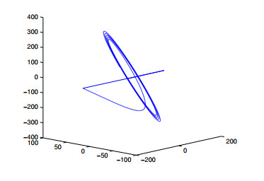
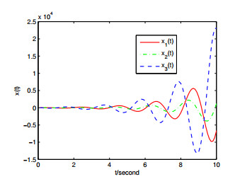
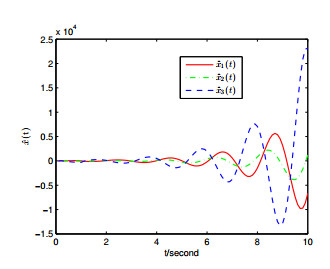
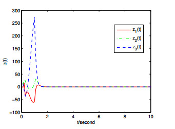
This paper investigates the master-slave synchronization of Lurie systems with time delay via the event-triggered control. Different from some state feedback control methods with a fixed sampling period or impulsive control with random sampling moments, the event-triggered control means that the controller is updated only if some event-triggering conditions are satisfied. A predefined triggering condition is provided by using the Lyapunov stability theory. Moreover, this condition is proved not to be commonplace. Finally, a numerical example is given to show the correctness of the proposed method.
- Master-slave synchronization,
- event-triggered control,
- Lurie system,
- time delay
Citation: Chao Ma, Tianbo Wang, Wenjie You. Master-slave synchronization of Lurie systems with time-delay based on event-triggered control[J]. AIMS Mathematics, 2023, 8(3): 5998-6008. doi: 10.3934/math.2023302

Related Papers:

Abstract

This paper investigates the master-slave synchronization of Lurie systems with time delay via the event-triggered control. Different from some state feedback control methods with a fixed sampling period or impulsive control with random sampling moments, the event-triggered control means that the controller is updated only if some event-triggering conditions are satisfied. A predefined triggering condition is provided by using the Lyapunov stability theory. Moreover, this condition is proved not to be commonplace. Finally, a numerical example is given to show the correctness of the proposed method.

References

[1]	H. Mkaouar, O. Boubaker, Chaos synchronization for master slave piecewise linear systems: application to Chua's circuit, Commun. Nonlinear Sci., 17 (2012), 1292–1302. https://doi.org/10.1016/j.cnsns.2011.07.027 doi: 10.1016/j.cnsns.2011.07.027
[2]	T. P. Chen, S. Amari, Stability of asymmetric Hopfield networks, IEEE T. Neural Networ., 12 (2001), 159–163. https://doi.org/10.1109/72.896806 doi: 10.1109/72.896806
[3]	C. Guzelis, L. Chua, Stability analysis of generalized celluar neural networks, Int. J. Circ. Theor. App., 21 (1993), 1–33. https://doi.org/10.1002/cta.4490210102 doi: 10.1002/cta.4490210102
[4]	M. E. Yalcin, J. A. K. Suykens, J. Vandewalle, Master-slave synchronization of Lur'e systems with time-delay, Int. J. Bifurcat. Chaos, 11 (2001), 1707–1722. https://doi.org/10.1142/S021812740100295X doi: 10.1142/S021812740100295X
[5]	Z. Tang, J. H. Park, J. W. Feng, Novel approaches to pin cluster synchronization on complex dynamical networks in Lur'e forms, Commun. Nonlinear Sci., 57 (2018), 422–438. https://doi.org/10.1016/j.cnsns.2017.10.010 doi: 10.1016/j.cnsns.2017.10.010
[6]	S. T. Qin, Q. Cheng, G. F. Chen, Global exponential stability o funcertain neural networks with discontinuous Lurie-type activation and mixed delays, Neurocomputing, 198 (2016), 12–19.
[7]	X. Wang, X. Z. Liu, K. She, S. M. Zhong, Finite-time lag synchronization of master-slave complex dynamical networks with unknown signal propagation delays, J. Franklin I., 354 (2017), 4913–4929. https://doi.org/10.1016/j.jfranklin.2017.05.004 doi: 10.1016/j.jfranklin.2017.05.004
[8]	K. B. Shi, Y. Y. Tang, X. Z. Liu, S. M. Zhong, Non-fragile sampled-data robust synchronization of uncertain delayed chaotic Lurie systems with randomly occurring controller gain fluctuation, ISA T., 66 (2017), 185–199. https://doi.org/10.1016/j.isatra.2016.11.002 doi: 10.1016/j.isatra.2016.11.002
[9]	C. Yin, S. M. Zhong, W. F. Chen, Design PD controller for master-slave synchronization of chaotic Lur'e systems with sector and slope restricted nonlinearities, Commun. Nonlinear Sci., 16 (2011), 1632–1639. https://doi.org/10.1016/j.cnsns.2010.05.031 doi: 10.1016/j.cnsns.2010.05.031
[10]	A. Loria, Master-slave synchronization of fourth-order L$\ddot{u}$ chaotic oscillators via linear output feedback, IEEE T. Circuits-II, 57 (2010), 213–217. https://doi.org/10.1109/TCSII.2010.2040303 doi: 10.1109/TCSII.2010.2040303
[11]	Y. Q. Wang, J. Q. Lu, J. L. Liang, J. D. Cao, M. Perc, Pinning synchronization of nonlinear coupled Lur'e networks under hybrid impulses, IEEE T. Circuits-II, 66 (2019), 432–436. https://doi.org/10.1109/TCSII.2018.2844883 doi: 10.1109/TCSII.2018.2844883
[12]	Y. B. Yu, F. L. Zhang, Q. S. Zhong, X. F. Liao, J. B. Yu, Impulsive control of Lurie systems, Comput. Math. Appl., 56 (2008), 2806–2813. https://doi.org/10.1016/j.camwa.2008.09.015 doi: 10.1016/j.camwa.2008.09.015
[13]	Q. Xiao, T. G. Huang, Z. G. Zeng, Synchronization of timescale-type nonautonomous neural networks with proportional delays, IEEE T. Syst. Man Cy., 52 (2022), 2167–2173. https://doi.org/10.1109/TSMC.2021.3049363 doi: 10.1109/TSMC.2021.3049363
[14]	J. Q. Lu, J. D. Cao, D. W. C. Ho, Adaptive stabilization and synchronization for chaotic Lur'e systems with time-varying delay, IEEE T. Circuits-I, 55 (2008), 1347–1356. https://doi.org/10.1109/TCSI.2008.916462 doi: 10.1109/TCSI.2008.916462
[15]	W. H. Chen, Z. P. Wang, X. M. Lu, On sampled-data control for master-slave synchronization of chaotic Lur'e systems, IEEE T. Circuits-II, 59 (2012), 515–519. https://doi.org/10.1109/TCSII.2012.2204114 doi: 10.1109/TCSII.2012.2204114
[16]	D. H. Ji, J. H. Park, S. C. Won, Master-slave synchronization of Lur'e systems with sector and slope restricted nonlinearities, Phys. Lett. A, 373 (2009), 1044–1050. https://doi.org/10.1016/j.physleta.2009.01.038 doi: 10.1016/j.physleta.2009.01.038
[17]	H. M. Guo, S. M. Zhong, F. Y. Gao, Design of PD controller for master-slave synchronization of Lur'e systems with time-delay, Appl. Math. Comput., 212 (2009), 86–93. https://doi.org/10.1016/j.amc.2009.01.080 doi: 10.1016/j.amc.2009.01.080
[18]	X. J. Su, X. X. Liu, P. Shi, Y. D. Song, Sliding mode control of hybrid switched systems via an event-triggered mechanism, Automatica, 90 (2018), 294–303. https://doi.org/10.1016/j.automatica.2017.12.033 doi: 10.1016/j.automatica.2017.12.033
[19]	X. Q. Xiao, L. Zhou, D. W. C. Ho, G. P. Lu, Event-triggered control of continuous-time switched linear systems, IEEE T. Automat. Contr., 64 (2019), 1710–1717. https://doi.org/10.1109/TAC.2018.2853569 doi: 10.1109/TAC.2018.2853569
[20]	D. X. Peng, X. D. Li, Leader-following synchronization of complex dynamic networks via event-triggered impulsive control, Neurocomputing, 412 (2020), 1–10. https://doi.org/10.1016/j.neucom.2020.05.071 doi: 10.1016/j.neucom.2020.05.071
[21]	J. Liu, H. Q. Wu, J. D. Cao, Event-triggered synchronization in fixed time for semi-Markov switching dynamical complex networks with multiple weights and discontinuous nonlinearity, Commun. Nonlinear Sci., 90 (2020), 105400. https://doi.org/10.1016/j.cnsns.2020.105400 doi: 10.1016/j.cnsns.2020.105400
[22]	M. Z. Wang, S. C. Wu, X. D. Li, Event-triggered delayed impulsive control for nonlinear systems with applications, J. Franklin I., 358 (2021), 4277–4291. https://doi.org/10.1016/j.jfranklin.2021.03.021 doi: 10.1016/j.jfranklin.2021.03.021
[23]	X. F. Fan, Z. S. Wang, Event-triggered sliding mode control for singular systems with disturbance, Nonlinear Anal.-Hybri., 40 (2021), 101011. https://doi.org/10.1016/j.nahs.2021.101011 doi: 10.1016/j.nahs.2021.101011
[24]	Y. Sun, P. Shi, C. C. Lim, Event-triggered sliding mode scaled consensus control for multi-agent systems, J. Franklin I., 359 (2022), 981–998. https://doi.org/10.1016/j.jfranklin.2021.12.007 doi: 10.1016/j.jfranklin.2021.12.007
[25]	W. Zhao, W. W. Yu, H. P. Zhang, Event-triggered optimal consensus tracking control for multi-agent systems with unknown internal states and disturbances, Nonlinear Anal.-Hybri., 33 (2019), 227–248. https://doi.org/10.1016/j.nahs.2019.03.003 doi: 10.1016/j.nahs.2019.03.003
[26]	W. H. Wu, L. He, J. P. Zhou, Z. X. Xuan, A. Sabri, Disturbance-term-based switching event-triggered synchronization control of chaotic Lurie systems subject to a joint performance guarantee, Commun. Nonlinear Sci., 115 (2022), 106774. https://doi.org/10.1016/j.cnsns.2022.106774 doi: 10.1016/j.cnsns.2022.106774
[27]	J. K. Tian, W. J. Xiong, F. Xu, Improved delay-partitioning method to stability analysis for neural networks with discrete and distributed time-varying delays, Appl. Math. Comput., 233 (2014), 152–164. https://doi.org/10.1016/j.amc.2014.01.129 doi: 10.1016/j.amc.2014.01.129
[28]	W. L. He, F. Qian, Q. L. Han, J. D. Cao, Synchronization error estimation and controller design for delayed Lur'e systems with parameter mismatches, IEEE T. Neur. Net. Lear., 23 (2012), 1551–1562. https://doi.org/10.1109/TNNLS.2012.2205941 doi: 10.1109/TNNLS.2012.2205941

Reader Comments

Your name:*

Email:*
© 2023 the Author(s), licensee AIMS Press. This is an open access article distributed under the terms of the Creative Commons Attribution License (http://creativecommons.org/licenses/by/4.0)