Modeling the dynamics of innate and adaptive immune response to Parkinson's disease with immunotherapy

Salma M. Al-Tuwairqi; Asma A. Badrah; Salma M. Al-Tuwairqi; Asma A. Badrah

doi:10.3934/math.2023093

AIMS Mathematics

2023, Volume 8, Issue 1: 1800-1832. doi: 10.3934/math.2023093

Previous Article Next Article

Research article

Modeling the dynamics of innate and adaptive immune response to Parkinson's disease with immunotherapy

Salma M. Al-Tuwairqi ^,,
Asma A. Badrah

Department of Mathematics, King Abdulaziz University, Jeddah, Saudi Arabia

Received: 31 July 2022 Revised: 22 September 2022 Accepted: 04 October 2022 Published: 25 October 2022
MSC : 34C60, 34D20, 34D23, 92D30

A mathematical model was built using delay differential equations to investigate the effect of active and passive immunotherapies in delaying the progression of Parkinson's Disease. The model described the dynamics between healthy and infected neurons and alpha-synuclein with innate and adaptive immune responses. The model was examined qualitatively and numerically. The qualitative analysis produced two equilibrium points. The local stability of the free and endemic equilibrium points was established depending on the basic reproduction number, $ R_0 $. Numerical simulations were executed to show the agreement with the qualitative results. Moreover, a sensitivity analysis on $ R_0 $ was conducted to examine the critical parameters in controlling $ R_0 $. We found that if treatment is administered in the early stages of the disease with short time delays, alpha-synuclein is combated, inhibiting activated microglia and T cells and preserving healthy neurons. It can be concluded that administering time of immunotherapies plays a significant role in hindering the advancement of Parkinson's disease.
- alpha-synuclein,
- Parkinson's disease,
- mathematical model,
- time delay,
- immunotherapy,
- stability
Citation: Salma M. Al-Tuwairqi, Asma A. Badrah. Modeling the dynamics of innate and adaptive immune response to Parkinson's disease with immunotherapy[J]. AIMS Mathematics, 2023, 8(1): 1800-1832. doi: 10.3934/math.2023093

Related Papers:

Abstract

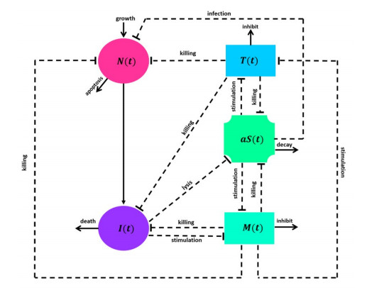
A mathematical model was built using delay differential equations to investigate the effect of active and passive immunotherapies in delaying the progression of Parkinson's Disease. The model described the dynamics between healthy and infected neurons and alpha-synuclein with innate and adaptive immune responses. The model was examined qualitatively and numerically. The qualitative analysis produced two equilibrium points. The local stability of the free and endemic equilibrium points was established depending on the basic reproduction number, $ R_0 $. Numerical simulations were executed to show the agreement with the qualitative results. Moreover, a sensitivity analysis on $ R_0 $ was conducted to examine the critical parameters in controlling $ R_0 $. We found that if treatment is administered in the early stages of the disease with short time delays, alpha-synuclein is combated, inhibiting activated microglia and T cells and preserving healthy neurons. It can be concluded that administering time of immunotherapies plays a significant role in hindering the advancement of Parkinson's disease.

References

[1]	M. J. Benskey, R. G. Perez, F. P. Manfredsson, The contribution of alpha synuclein to neuronal survival and function–Implications for Parkinson's disease, J. Neurochem., 137 (2016), 331–359, https://doi.org/10.1111/jnc.13570 doi: 10.1111/jnc.13570
[2]	S. Mehra, S. Sahay, S. K. Maji, $\alpha$-Synuclein misfolding and aggregation: Implications in Parkinson's disease pathogenesis, Biochim. Biophys. Acta Proteins Proteom., 1867 (2019), 890–908. https://doi.org/10.1016/j.bbapap.2019.03.001 doi: 10.1016/j.bbapap.2019.03.001
[3]	R. M. Meade, D. P. Fairlie, J. M. Mason, Alpha-synuclein structure and Parkinson's disease, Mol. Neurodegener., 14 (2019), 29. https://doi.org/10.1186/s13024-019-0329-1 doi: 10.1186/s13024-019-0329-1
[4]	A. D. Schwab, M. J. Thurston, J. Machhi, K. E. Olson, K. L. Namminga, H. E. Gendelman, et al., Immunotherapy for Parkinson's disease, Neurobiol. Dis., 137 (2020), 104760. https://doi.org/10.1016/j.nbd.2020.104760 doi: 10.1016/j.nbd.2020.104760
[5]	J. Shin, H. J. Kim, B. Jeon, Immunotherapy targeting neurodegenerative proteinopathies: $\alpha$-synucleinopathies and tauopathies, J. Movement Disorders, 13 (2020), 11–19. https://doi.org/10.14802/jmd.19057 doi: 10.14802/jmd.19057
[6]	H. J. Lee, E. D. Cho, K. W. Lee, J. H. Kim, S. G. Cho, S. J. Lee, Autophagic failure promotes the exocytosis and intercellular transfer of $\alpha$-synuclein, Exp. Mol. Med., 45 (2013), e22. https://doi.org/10.1038/emm.2013.45 doi: 10.1038/emm.2013.45
[7]	C. R. Overk, E. Masliah, Pathogenesis of synaptic degeneration in Alzheimer's disease and Lewy body disease, Biochem. Pharmacol., 88 (2014), 508–516. https://doi.org/10.1016/j.bcp.2014.01.015 doi: 10.1016/j.bcp.2014.01.015
[8]	A. Recasens, B. Dehay, J. Bové, I. Carballo-Carbajal, S. Dovero, A. Pérez-Villalba, et al., Lewy body extracts from parkinson disease brains trigger $\alpha$-synuclein pathology and neurodegeneration in mice and monkeys, Ann. Neurol., 75 (2014), 351–362. https://doi.org/10.1002/ana.24066 doi: 10.1002/ana.24066
[9]	Y. Chu, J. H. Kordower, The prion hypothesis of Parkinson's disease, Curr. Neurol. Neurosci. Rep., 15 (2015), 28. https://doi.org/10.1007/s11910-015-0549-x doi: 10.1007/s11910-015-0549-x
[10]	R. L. Mosley, J. A. Hutter-Saunders, D. K. Stone, H. E. Gendelman, Inflammation and adaptive immunity in parkinson's disease, Cold Spring Harbor Perspectives in Medicine, 2012, 1–18. https://doi.org/10.1101/cshperspect.a009381 doi: 10.1101/cshperspect.a009381
[11]	J. Y. Li, E. Englund, J. L. Holton, D. Soulet, P. Hagell, A. J. Lees, et al., Lewy bodies in grafted neurons in subjects with parkinson's disease suggest host-to-graft disease propagation, Nat. Med., 14 (2008), 501–503. https://doi.org/10.1038/nm1746 doi: 10.1038/nm1746
[12]	J. H. Kordower, Y. Chu, R. A. Hauser, T. B. Freeman, C. W. Olanow, Lewy body–like pathology in long-term embryonic nigral transplants in parkinson's disease, Nat. Med., 14 (2008), 504–506. https://doi.org/10.1038/nm1747 doi: 10.1038/nm1747
[13]	A. C. Hoffmann, G. Minakaki, S. Menges, R. Salvi, S. Savitskiy, A. Kazman, et al., Extracellular aggregated alpha synuclein primarily triggers lysosomal dysfunction in neural cells prevented by trehalose, Sci. Rep., 9 (2019), 1–18. https://doi.org/10.1038/s41598-018-35811-8 doi: 10.1038/s41598-018-35811-8
[14]	P. Desplats, H. J. Lee, E. J. Bae, C. Patrick, E. Rockenstein, L. Crews, et al., Inclusion formation and neuronal cell death through neuron-to-neuron transmission of $\alpha$-synuclein, Proc. Natl. Acad. Sci. U. S. A., 106 (2009), 13010–13015. https://doi.org/10.1073/pnas.0903691106 doi: 10.1073/pnas.0903691106
[15]	S. Kwon, M. Iba, C. Kim, E. Masliah, Immunotherapies for aging-related neurodegenerative diseases-emerging perspectives and new targets, Neurotherapeutics, 17 (2020), 935–954. https://doi.org/10.1007/s13311-020-00853-2 doi: 10.1007/s13311-020-00853-2
[16]	C. Arcuri, C. Mecca, R. Bianchi, I. Giambanco, R. Donato, The pathophysiological role of microglia in dynamic surveillance, phagocytosis and structural remodeling of the developing cns, Front. Mol. Neurosci., 10 (2017), 191. https://doi.org/10.3389/fnmol.2017.00191 doi: 10.3389/fnmol.2017.00191
[17]	T. Town, V. Nikolic, J. Tan, The microglial "activation" continuum: From innate to adaptive responses, J. Neuroinflammation, 2 (2005), 24. https://doi.org/10.1186/1742-2094-2-24 doi: 10.1186/1742-2094-2-24
[18]	V. Vedam-Mai, Harnessing the immune system for the treatment of parkinson's disease, Brain Res., 1758 (2021), 147308. https://doi.org/10.1016/j.brainres.2021.147308 doi: 10.1016/j.brainres.2021.147308
[19]	A. M. Schonhoff, G. P. Williams, Z. D. Wallen, D. G. Standaert, A. S. Harms, Chapter 6–innate and adaptive immune responses in parkinson's disease, Prog. Brain Res., 252 (2020), 169–216.
[20]	A. M. Jurga, M. Paleczna, K. Z. Kuter, Overview of general and discriminating markers of differential microglia phenotypes, Front. Cell. Neurosci., 14 (2020), 198. https://doi.org/10.3389/fncel.2020.00198 doi: 10.3389/fncel.2020.00198
[21]	E. J. Bae, H. J. Lee, E. Rockenstein, D. H. Ho, E. B. Park, N. Y. Yang, et al., Antibody-aided clearance of extracellular $\alpha$-synuclein prevents cell-to-cell aggregate transmission, J. Neurosci., 32 (2012), 13454–13469. https://doi.org/10.1523/JNEUROSCI.1292-12.2012 doi: 10.1523/JNEUROSCI.1292-12.2012
[22]	J. Y. Vargas, C. Grudina, C. Zurzolo, The prion-like spreading of $\alpha$-synuclein: From in vitro to in vivo models of Parkinson's disease, Ageing Res. Rev., 50 (2019), 89–101. https://doi.org/10.1016/j.arr.2019.01.012 doi: 10.1016/j.arr.2019.01.012
[23]	D. Chatterjee, J. H. Kordower, Immunotherapy in Parkinson's disease: Current status and future directions, Neurobiol. Dis., 132 (2019), 104587. https://doi.org/10.1016/j.nbd.2019.104587 doi: 10.1016/j.nbd.2019.104587
[24]	J. Cruse, R. Lewis, H. Wang, Immunology guidebook, Academic Press, 2004. https://doi.org/10.1016/B978-0-12-198382-6.X5022-5
[25]	F. A. Bonilla, H. C. Oettgen, Adaptive immunity, J. Allergy Clinical Immunology, 125 (2010), S33–S40. https://doi.org/10.1016/j.jaci.2009.09.017 doi: 10.1016/j.jaci.2009.09.017
[26]	F. Garretti, D. Agalliu, C. S. Lindestam Arlehamn, A. Sette, D. Sulzer, Autoimmunity in parkinson's disease: The role of $\alpha$-synuclein-specific T cells, Front. Immunol., 10 (2019), 303. https://doi.org/10.3389/fimmu.2019.00303 doi: 10.3389/fimmu.2019.00303
[27]	A. Lloret-Villas, T. M. Varusai, N. Juty, C. Laibe, N. Le Novere, H. Hermjakob, et al., The impact of mathematical modeling in understanding the mechanisms underlying neurodegeneration: Evolving dimensions and future directions, CPT: Pharmacometrics Syst. Pharmacol., 6 (2017), 73–86. https://doi.org/10.1002/psp4.12155 doi: 10.1002/psp4.12155
[28]	Y. Sarbaz, H. Pourakbari, A review of presented mathematical models in Parkinson's disease: Black- and gray-box models, Med. Biol. Eng. Comput., 54 (2016), 855–868. https://doi.org/10.1007/s11517-015-1401-9 doi: 10.1007/s11517-015-1401-9
[29]	I. K. Puri, L. Li, Mathematical modeling for the pathogenesis of alzheimer's disease, PloS One, 5 (2010), e15176. https://doi.org/10.1371/journal.pone.0015176 doi: 10.1371/journal.pone.0015176
[30]	W. Hao, A. Friedman, Mathematical model on Alzheimer's disease, BMC Syst. Biol., 10 (2016), 108. https://doi.org/10.1186/s12918-016-0348-2 doi: 10.1186/s12918-016-0348-2
[31]	I. A. Kuznetsov, A. V. Kuznetsov, What can trigger the onset of Parkinson's disease–A modeling study based on a compartmental model of $\alpha$-synuclein transport and aggregation in neurons, Math. Biosci., 278 (2016), 22–29. https://doi.org/10.1016/j.mbs.2016.05.002 doi: 10.1016/j.mbs.2016.05.002
[32]	I. A. Kuznetsov, A. V. Kuznetsov, Mathematical models of $\alpha$-synuclein transport in axons, Comput. Methods Biomech. Biomed. Eng., 19 (2016), 515–526. https://doi.org/10.1080/10255842.2015.1043628 doi: 10.1080/10255842.2015.1043628
[33]	K. Sneppen, L. Lizana, M. H. Jensen, S. Pigolotti, D. Otzen, Modeling proteasome dynamics in Parkinson's disease, Phys. Biol., 6 (2009), 036005. https://doi.org/10.1088/1478-3975/6/3/036005 doi: 10.1088/1478-3975/6/3/036005
[34]	A. Badrah, S. Al-Tuwairqi, Modeling the dynamics of innate immune response to parkinson disease with therapeutic approach, Phys. Biol., 19 (2022), 056004. https://doi.org/10.1088/1478-3975/ac8516 doi: 10.1088/1478-3975/ac8516
[35]	J. Yang, X. Wang, F. Zhang, A differential equation model of HIV infection of $CD_4^+$ T cells with delay, Discrete Dyn. Nat. Soc., 2008 (2008), 903678. https://doi.org/10.1155/2008/903678 doi: 10.1155/2008/903678
[36]	S. Çakan, Dynamic analysis of a mathematical model with health care capacity for COVID-19 pandemic, Chaos Solitons Fract., 139 (2020), 110033. https://doi.org/10.1016/j.chaos.2020.110033 doi: 10.1016/j.chaos.2020.110033
[37]	M. B. Finan, A first course in quasi-linear partial differential equations for physical sciences and engineering, 2019.
[38]	M. Martcheva, An introduction to mathematical epidemiology, New York: Springer, 2015. https://doi.org/10.1007/978-1-4899-7612-3
[39]	O. Nonthakorn, Biological models with time delay, PhD thesis, Worcester Polytechnic Institute, 2016.
[40]	C. Castillo-Chavez, Z. Feng, W. Huang, On the computation of $R_0$ and its role in global stability, Math. Approaches Emerg Re-emerg. Infect. Dis., 125 (2002), 229–250.
[41]	Z. S. Kifle, L. L. Obsu, Mathematical modeling for COVID-19 transmission dynamics: A case study in ethiopia, Results Phys., 105191. https://doi.org/10.1016/j.rinp.2022.105191

Reader Comments

Your name:*

Email:*
© 2023 the Author(s), licensee AIMS Press. This is an open access article distributed under the terms of the Creative Commons Attribution License (http://creativecommons.org/licenses/by/4.0)