A hyperchaos generated from Rabinovich system

Junhong Li; Ning Cui; Junhong Li; Ning Cui

doi:10.3934/math.2023071

AIMS Mathematics

2023, Volume 8, Issue 1: 1410-1426. doi: 10.3934/math.2023071

Previous Article Next Article

Research article

A hyperchaos generated from Rabinovich system

Junhong Li ,
Ning Cui ^,

School of Mathematics and Statistics, Hanshan Normal University, Chaozhou 521041, Guangdong, China

Received: 08 July 2022 Revised: 29 September 2022 Accepted: 13 October 2022 Published: 20 October 2022
MSC : 34K18, 65P20

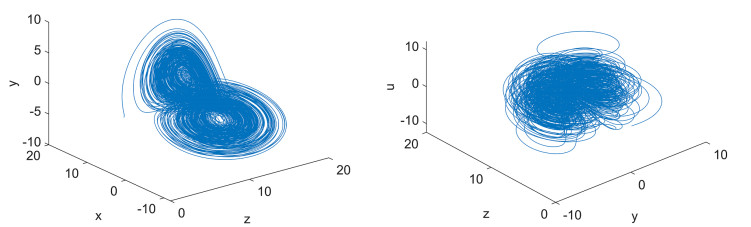
In this paper, we present a 4D hyperchaotic Rabinovich system which obtained by adding a linear controller to 3D Rabinovich system. Based on theoretical analysis and numerical simulations, the rich dynamical phenomena such as boundedness, dissipativity and invariance, equilibria and their stability, chaos and hyperchaos are studied. In addition, the Hopf bifurcation at the zero equilibrium point of the 4D Rabinovich system is investigated. The numerical simulations, including phase diagrams, Lyapunov exponent spectrum, bifurcations, power spectrum and Poincaré maps, are carried out in order to analyze and verify the complex phenomena of the 4D Rabinovich system.
- Rabinovich system,
- hyperchaos,
- Lyapunov exponents,
- bifurcation
Citation: Junhong Li, Ning Cui. A hyperchaos generated from Rabinovich system[J]. AIMS Mathematics, 2023, 8(1): 1410-1426. doi: 10.3934/math.2023071

Related Papers:

Abstract

In this paper, we present a 4D hyperchaotic Rabinovich system which obtained by adding a linear controller to 3D Rabinovich system. Based on theoretical analysis and numerical simulations, the rich dynamical phenomena such as boundedness, dissipativity and invariance, equilibria and their stability, chaos and hyperchaos are studied. In addition, the Hopf bifurcation at the zero equilibrium point of the 4D Rabinovich system is investigated. The numerical simulations, including phase diagrams, Lyapunov exponent spectrum, bifurcations, power spectrum and Poincaré maps, are carried out in order to analyze and verify the complex phenomena of the 4D Rabinovich system.

References

[1]	O. E. Rössler, An equation for hyperchaos, Phys. Lett. A, 71 (1979), 155–157. https://doi.org/10.1016/0375-9601(79)90150-6
[2]	C. Xiu, R. Zhou, S. Zhao, G. Xu, Memristive hyperchaos secure communication based on sliding mode control, Nonlinear Dyn., 104 (2021), 789–805. https://doi.org/10.1007/s11071-021-06302-9 doi: 10.1007/s11071-021-06302-9
[3]	M. Boumaraf, F. Merazka, Secure speech coding communication using hyperchaotic key generators for AMR-WB codec, Multimedia Syst., 27 (2021), 247–269. https://doi.org/10.1007/s00530-020-00738-6 doi: 10.1007/s00530-020-00738-6
[4]	D. Jiang, L. Liu, L. Zhu, X. Wang, X. Rong, H. Chai, Adaptive embedding: A novel meaningful image encryption scheme based on parallel compressive sensing and slant transform, Signal Proc., 188 (2021), 108220. https://doi.org/10.1016/j.sigpro.2021.108220 doi: 10.1016/j.sigpro.2021.108220
[5]	P. C. Rech, Chaos and hyperchaos in a Hopfield neural network, Neurocomputing, 74 (2011), 3361–3364. https://doi.org/10.1016/j.neucom.2011.05.016 doi: 10.1016/j.neucom.2011.05.016
[6]	H. Li, Z. Hua, H. Bao, L. Zhu, M. Chen, B. Bao, Two-dimensional memristive hyperchaotic maps and application in secure communication, IEEE T. Ind. Electron., 68 (2020), 9931–9940. https://doi.org/10.1109/TIE.2020.3022539 doi: 10.1109/TIE.2020.3022539
[7]	Y. Su, X. Wang, Characteristic analysis of new four-dimensional autonomous power system and its application in color image encryption, Multimedia Syst., 28 (2022), 553–571. https://doi.org/10.1007/s00530-021-00861-y doi: 10.1007/s00530-021-00861-y
[8]	Y. Si, H. Liu, Y. Chen, Constructing a 3D exponential hyperchaotic map with application to PRNG, Int. J. Bifurcat. Chaos, 32 (2022), 2250095. https://doi.org/10.1142/S021812742250095X doi: 10.1142/S021812742250095X
[9]	A. Chen, J. Lu, J. Lü, S. Yu, Generating hyperchaotic Lü attractor via state feedback control, Phys. A, 364 (2006), 103–110. https://doi.org/10.1016/j.physa.2005.09.039 doi: 10.1016/j.physa.2005.09.039
[10]	Z. Yan, Controlling hyperchaos in the new hyperchaotic Chen system, Appl. Math. Comput., 168 (2005), 1239–1250. https://doi.org/10.1016/j.amc.2004.10.016 doi: 10.1016/j.amc.2004.10.016
[11]	T. Gao, Z. Chen, Q. Gu, Z. Yuan, A new hyper-chaos generated from generalized Lorenz system via nonlinear feedback, Chaos Soliton. Fract., 35 (2008), 390–397. https://doi.org/10.1016/j.chaos.2006.05.030 doi: 10.1016/j.chaos.2006.05.030
[12]	H. Wang, X. Li X, A novel hyperchaotic system with infinitely many heteroclinic orbits coined, Chaos Soliton. Fract., 106 (2018), 5–15. https://doi.org/10.1016/j.chaos.2017.10.029 doi: 10.1016/j.chaos.2017.10.029
[13]	N. Nguyen, T. Bui, G. Gagnon, P. Giard, G. Kaddoum, Designing a pseudorandom bit generator with a novel five-dimensional-hyperchaotic system, IEEE T. Ind. Electron., 69 (2022), 6101–6110. https://doi.org/10.1109/TIE.2021.3088330 doi: 10.1109/TIE.2021.3088330
[14]	S. Emiroglu, A. Akgül, Y. Adıyaman, T. E. Gümüş, Y. Uyaroglu, M. A. Yalçın, A new hyperchaotic system from T chaotic system: Dynamical analysis, circuit implementation, control and synchronization, Circuit World, 48 (2021), 265–277. https://doi.org/10.1108/CW-09-2020-0223 doi: 10.1108/CW-09-2020-0223
[15]	A. S. Pikovski, M. I. Rabinovich, V. Y. Trakhtengerts, Onset of stochasticity in decay confinement of parametric instability, Sov. Phys. JETP, 7 (1978), 715–719.
[16]	J. Llibre, M. Messias, P. D. Silva, On the global dynamics of the Rabinovich system, J. Phys. A, 41 (2008), 275210. https://doi.org/10.1088/1751-8113/41/27/275210 doi: 10.1088/1751-8113/41/27/275210
[17]	V. A. Boichenko, G. A. Leonov, V. Reitmann, Dimension theory for ordinary differential equations, Vieweg+Teubner Verlag, Wiesbaden, 2005.
[18]	Y. Liu, Q. Yang, G. Pang, A hyperchaotic system from the Rabinovich system, J. Comput. Appl. Math., 234 (2010), 101–113. https://doi.org/10.1016/j.cam.2009.12.008 doi: 10.1016/j.cam.2009.12.008
[19]	Y. Liu, Circuit implementation and finite-time synchronization of the 4D Rabinovich hyperchaotic system, Nonlinear Dyn., 67 (2012), 89–96. https://doi.org/10.1007/s11071-011-9960-2 doi: 10.1007/s11071-011-9960-2
[20]	Z. Wei, P. Yu, W. Zhang, M. Yao, Study of hidden attractors, multiple limit cycles from Hopf bifurcation and boundedness of motion in the generalized hyperchaotic Rabinovich system, Nonlinear Dyn., 82 (2015), 131–141. https://doi.org/10.1007/s11071-015-2144-8 doi: 10.1007/s11071-015-2144-8
[21]	X. Tong, Y. Liu, M. Zhang, H. Xu, Z. Wang, An image encryption scheme based on hyperchaotic Rabinovich and exponential chaos maps, Entropy, 17 (2015), 181–196. https://doi.org/10.3390/e17010181 doi: 10.3390/e17010181
[22]	Z. Zhang, L. Huang, A new 5D Hamiltonian conservative hyperchaotic system with four center type equilibrium points, wide range and coexisting hyperchaotic orbits, Nonlinear Dynam., 108 (2022), 637–652. https://doi.org/10.1007/s11071-021-07197-2 doi: 10.1007/s11071-021-07197-2
[23]	S. Yan, X. Sun, Z. Song, Y. Ren, Dynamical analysis and bifurcation mechanism of four-dimensional hyperchaotic system, Eur. Phys. J. Plus, 137 (2022), 734. https://doi.org/10.1140/epjp/s13360-022-02943-w doi: 10.1140/epjp/s13360-022-02943-w
[24]	Z. Li, F. Zhang, X. Zhang, Y. Zhao, A new hyperchaotic complex system and its synchronization realization, Phys. Scripta, 96 (2021), 045208. https://doi.org/10.1088/1402-4896/abdf0c doi: 10.1088/1402-4896/abdf0c
[25]	X. D. Edmund, K. Charles, Routh-Hurwitz criterion in the examination of eigenvalues of a system of nonlinear ordinary differential equations, Phys. Rev. A, 35 (1987), 5288–5290. https://doi.org/10.1103/PhysRevA.35.5288 doi: 10.1103/PhysRevA.35.5288
[26]	J. Guckenheimer, P. Holmes, Nonlinear oscillations, dynamical systems and bifurcations of vector fields, J. Appl. Mech., 51 (1984), 947. https://doi.org/10.1115/1.3167759 doi: 10.1115/1.3167759
[27]	B. Elizabeth, J. Gayathri, S. Subashini, A. Prakash, Hide: Hyperchaotic image encryption using DNA computing, J. Real-Time Image Proc., 19 (2022), 429–443. https://doi.org/10.1007/s11554-021-01194-9 doi: 10.1007/s11554-021-01194-9
[28]	S. Sajjadi, D. Baleanu, A. Jajarmi, H. Pirouz, A new adaptive synchronization and hyperchaos control of a biological snap oscillator, Chaos Soliton. Fract., 138 (2020), 109919. https://doi.org/10.1016/j.chaos.2020.109919 doi: 10.1016/j.chaos.2020.109919

Reader Comments

Your name:*

Email:*
© 2023 the Author(s), licensee AIMS Press. This is an open access article distributed under the terms of the Creative Commons Attribution License (http://creativecommons.org/licenses/by/4.0)