Reflexive edge strength of convex polytopes and corona product of cycle with path

Kooi-Kuan Yoong; Roslan Hasni; Gee-Choon Lau; Muhammad Ahsan Asim; Ali Ahmad; Kooi-Kuan Yoong; Roslan Hasni; Gee-Choon Lau; Muhammad Ahsan Asim; Ali Ahmad

doi:10.3934/math.2022657

AIMS Mathematics

2022, Volume 7, Issue 7: 11784-11800. doi: 10.3934/math.2022657

Previous Article Next Article

Research article

Reflexive edge strength of convex polytopes and corona product of cycle with path

1.
Special Interest Group on Modelling and Data Analytics (SIGMDA), Faculty of Ocean Engineering Technology and Informatics, Universiti Malaysia Terengganu, Terengganu, Malaysia
2.
Faculty of Computer and Mathematical Sciences, Universiti Teknologi MARA (Segamat Campus), Johor, Malaysia
3.
College of Computer Sciences and Information Technology, Jazan University, Jazan, Saudi Arabia

Received: 25 December 2021 Revised: 16 February 2022 Accepted: 21 February 2022 Published: 18 April 2022
MSC : 05C78, 05C38

For a graph $G$ , we define a total $k$ -labeling $\varphi$ is a combination of an edge labeling $\varphi_e(x)\to\{1, 2, \ldots, k_e\}$ and a vertex labeling $\varphi_v(x) \to \{0, 2, \ldots, 2k_v\}$ , such that $\varphi(x) = \varphi_v(x)$ if $x\in V(G)$ and $\varphi(x) = \varphi_e(x)$ if $x\in E(G)$ , then $k = \, \mbox{max}\, \{k_e, 2k_v\}$ . The total $k$ -labeling $\varphi$ is an edge irregular reflexive $k$ -labeling of $G$ if every two different edges $xy$ and $x^\prime y^\prime$ , the edge weights are distinct. The smallest value $k$ for which such labeling exists is called a reflexive edge strength of $G$ . In this paper, we focus on the edge irregular reflexive labeling of antiprism, convex polytopes $\mathcal D_{n}$ , $\mathcal R_{n}$ , and corona product of cycle with path. This study also leads to interesting open problems for further extension of the work.

Keywords:

Citation: Kooi-Kuan Yoong, Roslan Hasni, Gee-Choon Lau, Muhammad Ahsan Asim, Ali Ahmad. Reflexive edge strength of convex polytopes and corona product of cycle with path[J]. AIMS Mathematics, 2022, 7(7): 11784-11800. doi: 10.3934/math.2022657

Related Papers:

[1]	Mohammad Esmael Samei, Lotfollah Karimi, Mohammed K. A. Kaabar . To investigate a class of multi-singular pointwise defined fractional $q$ –integro-differential equation with applications. AIMS Mathematics, 2022, 7(5): 7781-7816. doi: 10.3934/math.2022437
[2]	Asghar Ahmadkhanlu, Hojjat Afshari, Jehad Alzabut . A new fixed point approach for solutions of a $p$ -Laplacian fractional $q$ -difference boundary value problem with an integral boundary condition. AIMS Mathematics, 2024, 9(9): 23770-23785. doi: 10.3934/math.20241155
[3]	Reny George, Sina Etemad, Fahad Sameer Alshammari . Stability analysis on the post-quantum structure of a boundary value problem: application on the new fractional $(p, q)$ -thermostat system. AIMS Mathematics, 2024, 9(1): 818-846. doi: 10.3934/math.2024042
[4]	Idris Ahmed, Sotiris K. Ntouyas, Jessada Tariboon . Separated boundary value problems via quantum Hilfer and Caputo operators. AIMS Mathematics, 2024, 9(7): 19473-19494. doi: 10.3934/math.2024949
[5]	Abdelatif Boutiara, Mohamed Rhaima, Lassaad Mchiri, Abdellatif Ben Makhlouf . Cauchy problem for fractional ${(p, q)}$ -difference equations. AIMS Mathematics, 2023, 8(7): 15773-15788. doi: 10.3934/math.2023805
[6]	Donny Passary, Sotiris K. Ntouyas, Jessada Tariboon . Hilfer fractional quantum system with Riemann-Liouville fractional derivatives and integrals in boundary conditions. AIMS Mathematics, 2024, 9(1): 218-239. doi: 10.3934/math.2024013
[7]	Khalid K. Ali, K. R. Raslan, Amira Abd-Elall Ibrahim, Mohamed S. Mohamed . On study the fractional Caputo-Fabrizio integro differential equation including the fractional q-integral of the Riemann-Liouville type. AIMS Mathematics, 2023, 8(8): 18206-18222. doi: 10.3934/math.2023925
[8]	Nichaphat Patanarapeelert, Jiraporn Reunsumrit, Thanin Sitthiwirattham . On nonlinear fractional Hahn integrodifference equations via nonlocal fractional Hahn integral boundary conditions. AIMS Mathematics, 2024, 9(12): 35016-35037. doi: 10.3934/math.20241667
[9]	Reny George, Sina Etemad, Ivanka Stamova, Raaid Alubady . Existence of solutions for $[\mathtt{p},\mathtt{q}]$ -difference initial value problems: application to the $[\mathtt{p},\mathtt{q}]$ -based model of vibrating eardrums. AIMS Mathematics, 2025, 10(2): 2321-2346. doi: 10.3934/math.2025108
[10]	Changlong Yu, Jufang Wang, Huode Han, Jing Li . Positive solutions of IBVPs for $q$ -difference equations with $p$ -Laplacian on infinite interval. AIMS Mathematics, 2021, 6(8): 8404-8414. doi: 10.3934/math.2021487

Abstract

1. Introduction

In the theory of quantum groups, the quantum universal enveloping algebra of three-dimensional simple Lie algebras $\mathfrak{sl}_2$ plays an important role ^[1]. In 1983, the one-parameter quantized enveloping algebra ${U_q}(\mathfrak{sl}_2)$ was introduced by Kulish and Reshetikhin in the context of the Yang-Baxter equation for the integrable statistical models in the quantum inverse scattering method, and later its Hopf algebraic structure was discovered by Sklyanin ^[1,2,3]. A few years later, Drinfeld and Jimbo ^[4,5,6,7] independently discovered quantized enveloping algebras with higher ranks of complex simple-Lie algebras, which are quasi-triangular Hopf algebras. When $q$ is not a root of unity, the representation theory of ${U_q}(\mathfrak{sl}_2)$ is very similar to that of the Lie algebra $\mathfrak{sl}_2$ , and has been basically solved. However, when $q$ is a root of unity, the quantum group ${U_q}(\mathfrak{sl}_2)$ will become very complex. Many authors study representations of ${U_q}(\mathfrak{sl}_2)$ when $q$ is a root of unity, and get some interesting results, see ^[8,9,10] for example.

In 2020, Aziziheris et al. ^[11] defined the classical Lie algebra $\mathfrak{sl}^{*}_2(\mathbb{C})$ based on a new associative multiplication on the $2 \times 2$ matrix, and then obtained a new type quantum group $U_{q}(\mathfrak{sl}^{*}_2)$ . In ^[12], Xu and Chen investigated the above new type quantum group $U_{q}(\mathfrak{sl}^{*}_2)$ and classified its all Hopf PBW-deformations in which the classical Drinfeld-Jimbo quantum group $U_q(\mathfrak{sl}_2)$ was almost the unique nontrivial one. In ^[13], the authors defined a new type restricted quantum group $\overline{U}_{q}(\mathfrak{sl}^{*}_2)$ and determined its Hopf PBW-deformations $\overline{U}_{q}(\mathfrak{sl}^{*}_2, \kappa)$ in which $\overline{U}_{q}(\mathfrak{sl}^{*}_2, 0) = \overline{U}_{q}(\mathfrak{sl}^{*}_2)$ and the classical restricted Drinfeld-Jimbo quantum group $\overline{U}_{q}(\mathfrak{sl}_2)$ was included. They showed that $\overline{U}_{q}(\mathfrak{sl}^{*}_2)$ was a basic Hopf algebra, then uniformly realize $\overline{U}_{q}(\mathfrak{sl}^{*}_2)$ and $\overline{U}_{q}(\mathfrak{sl}_2)$ via some quotients of (deformed) preprojective algebras corresponding to the Gabriel quiver of $\overline{U}_{q}(\mathfrak{sl}^{*}_2)$ .

One of the basic problems in the theory of quantum groups is to decompose a tensor product of modules into a direct sum of indecomposable ones and hence to elucidate the structure of the corresponding fusion rule algebra. In ^[8], Suter decomposed the restricted quantum universal enveloping algebra ${U_q}(\mathfrak{sl}_2)$ in a canonical way into a direct sum of indecomposable left (or right) ideals. The indecomposable finite-dimensional ${U_q}(\mathfrak{sl}_2)$ -modules were classified and the tensor products of two simple modules, simple and projective modules were decomposed into indecomposable ones. Su and Yang ^[10] accurately characterized the structure of the representation ring of the restricted quantum group $\overline{U}_{q}(\mathfrak{sl}_2)$ when $q$ is a primitive $2p$ -th $(p \ge 2)$ root of unity. In ^[14], the authors classified all the finite dimensional indecomposable $D(n)$ modules, and then gave the tensor product decomposition formulas between two indecomposables, at last described the representation ring by generators and relations clearly. In ^[15], for a class of $2n^2$ dimensional semisimple Hopf algebras $H_{2n^2}$ , the authors classified all irreducible $H_{2n^2}$ -modules, established the decomposition formulas of the tensor product of two irreducible $H_{2n^2}$ -modules and described the Grothendieck rings $r(H_{2n^2})$ by generators and relations explicitly. In the present paper, we will consider the decomposition of tensor products and try to describe the projective class ring of $\overline{U}_{q}(\mathfrak{sl}^{*}_2)$ .

The paper is organized as follows. In Section 2, we recall the definition of the new type restricted quantum group $\overline{U}_{q}(\mathfrak{sl}^{*}_2)$ and its Hopf algebra structure, and some preliminaries used in the following sections. In Section 3, we construct the principal indecomposable projective module $P_j$ through the primitive orthogonal idempotents of $\overline{U}_{q}(\mathfrak{sl}^{*}_2)$ , and then study its composition series, radical series, socle series and some other related properties. In Section 4, we give the decomposition formulas of tensor products between two simple modules, two indecomposable projective modules and a simple module and an indecomposable projective module of $\overline{U}_{q}(\mathfrak{sl}^{*}_2)$ . Furthermore, we describe the projective class ring by generators and relations explicitly.

Throughout the paper, we work over the complex field $\mathbb{C}$ . The notations $\mathbb{Z}$ and $\mathbb {Z}^{\geq 0}$ denote the set of all integers, and the set of all nonnegative integers respectively.

2. **The restricted quantum group $\overline{U}_{q}(\mathfrak{sl}^{*}_2)$**

Fix an integer $n\geq 3\; (n\neq 4)$ . From now on, we always assume that $q$ is a primitive $n$ -th root of unity, and

$\begin{eqnarray*} d = \left\{ \begin{array}{ll} n, &{\rm if}\; n\; {\rm is\; odd}, \\ \frac{n}{2}, &{\rm if}\; n\; {\rm is\; even}. \end{array} \right. \end{eqnarray*}$

First, we recall the definition of the new type restricted quantum group $\overline{U}_{q}(\mathfrak{sl}^{*}_2)$ and some properities as follows.

Definition 2.1. ^[13] The restricted quantum algebra $\overline{U}_{q}(\mathfrak{sl}^{*}_2)$ is an associative unital algebra generated by $K, K^{-1},$ $E,$ $F$ and subject to the following relations

$\begin{eqnarray*} && K K^{-1} = K^{-1} K = 1, \quad K^{d} = 1, \quad E^d = F^d = 0, \\ && KE = q^2EK, \quad KF = q^{-2}FK, \quad EF = FE. \end{eqnarray*}$

Lemma 2.2. ^[13] ${\rm (1)}$ The set $\left\{ F^i K^k E^j | i, j, k\in \mathbb{Z}, 0\leq i, j, k < d \right\}$ is a basis of $\overline{U}_{q}(\mathfrak{sl}^{*}_2),$ and the dimension of $\overline{U}_{q}(\mathfrak{sl}^{*}_2)$ is $d^3$ .

${\rm (2)}$ $\overline{U}_{q}(\mathfrak{sl}^{*}_2)$ is a Hopf algebra with coproduct $\Delta$ , counit $\varepsilon$ and antipode $S$ defined by

$\Delta(K) = K\otimes K, \ \ \Delta(E) = E\otimes K+1\otimes E, \ \ \Delta(F) = F\otimes 1+K^{-1}\otimes F,$

$\varepsilon(E) = 0, \ \ \varepsilon(F) = 0, \ \ \varepsilon(K) = \varepsilon(K^{-1}) = 1,$

$S(E) = -EK^{-1}, \ \ S(F) = -KF, \ \ S(K) = K^{-1}.$

${\rm (3)}$ $\overline{U}_{q}(\mathfrak{sl}^{*}_2)$ is a pointed, basic but not semisimple Hopf algebra.

Lemma 2.3. ^[13] Let $M$ be a finite dimensional simple $\overline{U}_{q}(\mathfrak{sl}^{*}_2)$ -module. Then ${\rm dim}(M) = 1$ and the module structure on $M = \mathbb{C} v_0$ can be given as follows:

$\begin{eqnarray} K v_0 = q^{l} v_0, \quad E v_0 = F v_0 = 0, \end{eqnarray}$

(2.1)

where $l\in \{0, 1, \cdots, d-1\}$ when $n$ is odd, $l \in \{0, 2, \cdots, {2(d-1)}\}$ when $n$ is even.

Lemma 2.4. ^[13] For any $i \in \mathbb{Z}_d$ , set $\epsilon_i = \frac{1}{d}\sum\limits_{l = 0}^{d - 1} {{q^{ - 2il}}{K^l}}$ . Obviously one has

${\epsilon _i}K = {q^{2i}}{\epsilon _i}, \; {\epsilon _i}E = E{\epsilon _{i - 1}}, \; {\epsilon _i}F = F{\epsilon _{i + 1}}.$

$\{ {\epsilon_i}|i \in {\mathbb{Z}_d}\}$ is a complete set of primitive orthogonal idempotents of $\overline{U}_{q}(\mathfrak{sl}^{*}_2)$ .

3. **The projective representations of the restricted quantum group $\overline{U}_{q}(\mathfrak{sl}^{*}_2)$**

Using the primitive orthogonal idempotents $\{ {\epsilon_i}|i \in {\mathbb{Z}_d}\}$ of $\overline{U}_{q}(\mathfrak{sl}^{*}_2)$ , one has

$\overline{U}_{q}(\mathfrak{sl}^{*}_2) = \overline{U}_{q}(\mathfrak{sl}^{*}_2){\epsilon_0} \oplus \overline{U}_{q}(\mathfrak{sl}^{*}_2){\epsilon_1} \oplus \cdots \oplus \overline{U}_{q}(\mathfrak{sl}^{*}_2){\epsilon_{d - 1}}.$

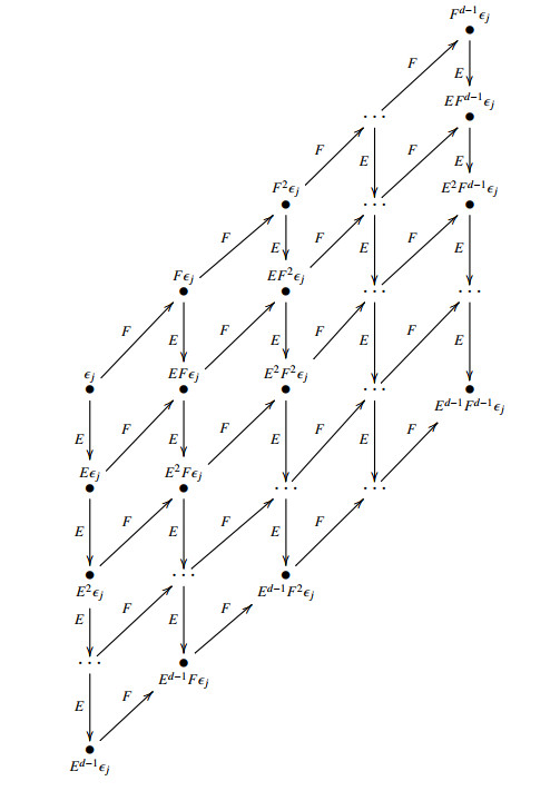
Let $P_j = \overline{U}_{q}(\mathfrak{sl}^{*}_2){\epsilon_j}$ , then $\{ P_j| j\in \mathbb{Z}_d\}$ is the set of the nonisomorphic principal indecomposable projective modules of $\overline{U}_{q}(\mathfrak{sl}^{*}_2)$ . As in ^[8], $P_j$ can be showed in Figure 1.

Figure 1. The structure of

$P_j$ .

DownLoad: Full-Size Img PowerPoint

Each point represents a one-dimensional vector space generated by the vector at that point, the downward arrows indicate the left action of $E$ , the right-oblique upward arrows indicate the left action of $F$ . shows that there are $d^2$ black dots, so the dimension of $P_j$ is $d^2$ .

From , it is easy to see that if we delete one point and the arrows connecting it at a time, from left to right, and from top to bottom, then we get a modules series, in which the former module modulo the next one is a 1-dimensional simple module. Therefore, we obtain the composition series of $P_j$ as follows.

Proposition 3.1. The principal indecomposable projective module $P_j\; (j \in \mathbb{Z}_d)$ has the following composition series:

$P_j = M_{0}^j\supset M_{1}^j\supset M_{2}^j\supset\cdots \supset M_{d^2}^j = 0,$

where for all $i \in \{ 0, 1, \ldots, d - 1\}$ ,

$\begin{eqnarray*} {M_i^j} & = &\mathop {\mathop \bigoplus \limits_{0 \le k < d} }\limits_{1 \le l < d} \mathbb{C}{E^k}{F^l}{\epsilon_j} \oplus \mathop \bigoplus \limits_{i \le k < d} \mathbb{C}{E^k}{\epsilon_j}, \\ {M_{d + i}^j} & = &\mathop {\mathop \bigoplus \limits_{0 \le k < d} }\limits_{2 \le l < d} \mathbb{C}{E^k}{F^l}{\epsilon_j} \oplus \mathop \bigoplus \limits_{i \le k < d} \mathbb{C}{E^k}F{\epsilon_j}, \\ & \vdots & \\ {M_{{d^2} - d+i}^j} & = & \mathop \bigoplus \limits_{i \le k < d} \mathbb{C}{E^k}{F^{d - 1}}{\epsilon_j}.\\ \end{eqnarray*}$

We can make the figures of ${M_1^j}$ and ${M_2^j}$ as follows (see Figures 2 and 3):

Figure 2. The structure of

$M_1^j$ .

DownLoad: Full-Size Img PowerPoint

Figure 3. The structure of

$M_2^j$ .

DownLoad: Full-Size Img PowerPoint

Proposition 3.2. The principal indecomposable projective module $P_j$ has a radical series as follows:

${P_j}\supset {\rm{ra}}{{\rm{d}}}(P_j)\supset {\rm{ra}}{{\rm{d}}^2}(P_j)\supset\cdots \supset {\rm{ra}}{{\rm{d}}^{2d-1}}(P_j) = 0,$

for all $i \in \{ 0, 1, \ldots, 2d - 1\},$

${\rm{ra}}{{\rm{d}}^i}({P_j}) = \mathop {\mathop \bigoplus \limits_{0 \le k, l < d} }\limits_{i \le k + l} \mathbb{C}{E^k}{F^l}{\epsilon_j}.$

Proof. Recall that ${\rm{rad}}({P_j})$ is exactly the intersection of all the maximal submodules of ${P_j}$ , and $P_j$ has a unique maximal submodule $M_1^j$ , so that ${\rm{rad}}({P_j}) = M_1^j$ , the figure is shown as before. ${\rm{ra}}{{\rm{d}}^2}({P_j})$ is the intersection of the maximal submodules of ${\rm{rad}}({P_j})$ , and is the submodule obtained by removing $\mathbb{C}{E}{\epsilon_j}$ and $\mathbb{C}{F}{\epsilon_j}$ and the connecting arrows, as shown in . Proceed this way, we have ${\rm{ra}}{{\rm{d}}^{2d - 2}}({P_j}) = \mathbb{C}{E^{d - 1}}{F^{d - 1}}{\epsilon_j}$ , ${\rm{ra}}{{\rm{d}}^{2d - 1}}({P_j}) = 0.$ □

Figure 4. The structure of

${\rm{ra}}{{\rm{d}}^2}(P_j)$ .

DownLoad: Full-Size Img PowerPoint

Proposition 3.3. The principal indecomposable projective module $P_j$ has a socle series as follows:

$0 = {\rm{so}}{{\rm{c}}^0}(P_j) \subset {\rm{so}}{{\rm{c}}}(P_j)\subset {\rm{so}}{{\rm{c}}^2}(P_j)\subset\cdots \subset {\rm{so}}{{\rm{c}}^{2d-1}}(P_j) = {P_j},$

for all $i \in \{ 0, 1, \ldots, 2d - 1\},$

${\rm{so}}{{\rm{c}}^i}({P_j}) = \mathop {\mathop \bigoplus \limits_{0 \le k, l < d} }\limits_{2d - 1 - i \le k + l} \mathbb{C}{E^k}{F^l}{\epsilon_j}.$

Proof. Recall that for $i\in \mathbb {Z}^{\geq 0}$ , ${\rm{so}}{{\rm{c}}^i}(P_j)$ is defined inductively as follows: ${\rm{so}}{{\rm{c}}^0}(P_j) = 0$ , and if ${\rm{so}}{{\rm{c}}^i}(P_j)$ is already defined and $p: P_j\rightarrow {\rm{so}}{\rm{c}}(P_j)$ denotes the canonical epimorphism, we get ${\rm{so}}{{\rm{c}}^{i+1}}(P_j) = p^{-1}({\rm{so}}{\rm{c}}(P_j/{\rm{so}}{{\rm{c}}^i}(P_j)))$ . Thus, by the definition, we have ${\rm{so}}{{\rm{c}}^0}(P_j) = 0$ , and as $P_j$ has only one simple submodule $\mathbb{C}E^{d-1}F^{d-1}{\epsilon_j}$ , so ${\rm{so}}{{\rm{c}}}(P_j) = \mathbb {C}E^{d-1}F^{d-1}{\epsilon_j}$ . Inductively, we have ${\rm{so}}{{\rm{c}}^2}(P_j) = \mathbb{C}E^{d-1}F^{d-1}{\epsilon_j} \oplus \mathbb{C}E^{d-1}F^{d-2}{\epsilon_j} \oplus \mathbb{C}E^{d-2}F^{d-1}{\epsilon_j};$ and we obtain a general expression of the socle series of the module $P_j$ as ${\rm{so}}{{\rm{c}}^i}({P_j}) = \mathop {\mathop \bigoplus \limits_{0 \le k, l < d} }\limits_{2d - 1 - i \le k + l} \mathbb{C}{E^k}{F^l}{\epsilon_j}$ , where $i \in \{ 0, 1, \ldots, 2d - 1\}$ . □

More intuitively, we can draw the figures ${\rm{so}}{{\rm{c}}}(P_j), \; {\rm{so}}{{\rm{c}}^2}(P_j), \; {\rm{so}}{{\rm{c}}^3}(P_j)$ as follows (see Figure 5):

Figure 5. The structures of

${\rm{so}}{{\rm{c}}}(P_j)$ ,

${\rm{so}}{{\rm{c}}^2}(P_j)$ and

${\rm{so}}{{\rm{c}}^3}(P_j)$ .

DownLoad: Full-Size Img PowerPoint

Observe the radical series and socle series of $P_j$ , it is easy to see that

${\rm{so}}{{\rm{c}}^s}(P_j) = {\rm{ra}}{{\rm{d}}^t}(P_j),$

where $s+t = 2d-1, s, t\in\{0, 1, \cdots 2d-1\}$ , and the length of the radical series(resp., the socle series) is $2d-1$ .

Note that ${\dim _\mathbb{C}}{\epsilon_i}{\overline{U}_{q}(\mathfrak{sl}^{*}_2)}{\epsilon_{j}} = d$ , we have

Proposition 3.4. (1) The dimensional vector of $P_j$ is

${\bf{dim}}\; P_j = {\left[ {\begin{array}{*{20}{c}} d, &d, \cdots , &d \end{array}} \right]^T}.$

(2) The $Cartan$ matrix of the algebra $\overline{U}_{q}(\mathfrak{sl}^{*}_2)$ is

$\left( {\begin{array}{*{20}{c}} d&d&\cdots&d\\ d&d&\cdots&d\\ \vdots & \vdots & \ddots & \vdots\\ d&d&\cdots&d \end{array}}\right) \in {\mathbb{M}_n}(\mathbb{Z}).$

4. **The projective class ring of $\overline{U}_{q}(\mathfrak{sl}^{*}_2)$**

Let $H$ be a finite dimensional Hopf algebra and $M$ and $N$ be two finite dimensional $H$ -modules. Then $M\otimes N$ is also a $H$ -module defined by

$h\cdot (m\otimes n) = \sum\limits_{(h)} h_{(1)}\cdot m\otimes h_{(2)}\cdot n$

for all $h\in H$ and $m\in M, n\in N$ , where $\Delta(h) = \sum_{(h)}h_{(1)}\otimes h_{(2)}.$ By the Krull-Schmidt Theorem, any finite dimensional $H$ -module can be decomposed into a direct sum of indecomposable $H$ -modules.

Now we consider the tensor products of two irreducible $\overline{U}_{q}(\mathfrak{sl}^{*}_2)$ -modules.

From Lemma 2.3, we know that for $\overline{U}_{q}(\mathfrak{sl}^{*}_2)$ there are $d$ non-isomorphic simple modules $S_i = \mathbb{C}v_i, i \in \{ 0, 1, \ldots, d - 1\}$ . Specifically, the module structure is:

$E\cdot v_i = \; F\cdot v_i = 0, \; K\cdot v_i = q^{2i} v_i.$

We have the following theorem:

Theorem 4.1. $S_{i}\otimes S_{j}\cong S_{(i+j){(\mathit{\text{mod}}\; d)}}, \; (0 \le i, j \le d - 1).$

Proof. Suppose that $S_i$ and $S_j$ are two simple modules of $\overline{U}_{q}(\mathfrak{sl}^{*}_2)$ , with basis $v_{i}, \; v_{j}$ respectively. Then $S_{i}\otimes S_{j}$ is also a $\overline{U}_{q}(\mathfrak{sl}^{*}_2)$ -module, with basis $v_{i}\otimes v_{j}$ and the actions of the generators are as follows

$\begin{eqnarray*} &&E \cdot ({v_i} \otimes {v_j}) = (E \otimes K + 1 \otimes E)({v_i} \otimes {v_j}) = 0, \\ &&F \cdot ({v_i} \otimes {v_j}) = (F \otimes 1 + {K^{ - 1}} \otimes F)({v_i} \otimes {v_j}) = 0, \\ &&K \cdot ({v_i} \otimes {v_j}) = (K \otimes K)({v_i} \otimes {v_j}) = {q^{2(i + j)}}{v_i} \otimes {v_j}. \end{eqnarray*}$

Therefore $S_{i}\otimes S_{j}\cong {S_{(i+j)(\text {mod}\; d)}}, \; (0 \le i, j \le d - 1).$ □

For the tensor products of a simple module with a projective module, we have

Theorem 4.2. $S_{i}\otimes P_{j}\cong P_{(i+j){(\mathit{\text{mod}}\; d)}} \cong P_{j}\otimes S_{i}, \; 0\leq i, j\leq d-1.$

Proof. Note that the basis of ${P_j}$ is $\left\{ {{E^k}{F^l}{\epsilon_j}|0 \le k, l \le d - 1} \right\}$ , let

$l_{1} = \epsilon_j, \; l_{2} = E\epsilon_j, \; \cdots, \; l_d = E^{d-1}\epsilon_j,$

$l_{d+1} = F\epsilon_j, \; l_{d+2} = EF\epsilon_j, \cdots, \; l_{2d} = E^{d-1}F\epsilon_j, \cdots,$

$l_{d^2-d+1} = F^{d-1}\epsilon_j, \; l_{d^2-d+2} = EF^{d-1}\epsilon_j, \cdots, \; l_{d^2} = E^{d-1}F^{d-1}\epsilon_j.$

Then the matrix of $K$ on the basis of $l_{1}, l_{2}, \cdots, l_{d}, l_{d+1}, l_{d+2}, \cdots, l_{2d}, \cdots, l_{d^2-d+1}, l_{d^2-d+2}, \cdots, l_{d^2}$ is

${A_1} = {\left( {\begin{array}{*{20}{c}} {{A_1^1}}&0& \cdots &0\\ 0&{{A_1^2}}& \cdots &0\\ \vdots & \vdots & \ddots & \vdots \\ 0&0& \cdots &{{A_1^d}} \end{array}} \right)_{{d^2} \times {d^2}}},$

where

${A_1^1} = {\left( {\begin{array}{*{20}{c}} {{q^{2j}}}&0& \cdots &0\\ 0&{{q^{2j + 2}}}& \cdots &0\\ \vdots & \vdots & \ddots & \vdots \\ 0&0& \cdots &{{q^{2j + 2d - 2}}} \end{array}} \right)_{d \times d}},$

${A_1^2} = {\left( {\begin{array}{*{20}{c}} {{q^{2j - 2}}}&0& \cdots &0\\ 0&{{q^{2j}}}& \cdots &0\\ \vdots & \vdots & \ddots & \vdots \\ 0&0& \cdots &{{q^{2j + 2d - 4}}} \end{array}} \right)_{d \times d}},$

$\vdots$

${A_1^d} = {\left( {\begin{array}{*{20}{c}} {{q^{2j - 2d + 2}}}&{}&{}&{}\\ {}&{{q^{2j - 2d + 4}}}&{}&{}\\ {}&{}& \ddots &{}\\ {}&{}&{}&{{q^{2j}}} \end{array}} \right)_{d \times d}}.$

The matrix of $E$ acting on this basis is

${B_1} = {\left( {\begin{array}{*{20}{c}} {{N}}&0& \cdots &0\\ 0&{{N}}& \cdots &0\\ \vdots & \vdots & \ddots & \vdots \\ 0&0& \cdots &{{N}} \end{array}} \right)_{{d^2} \times {d^2}}},$

where

${N} = {\left( {\begin{array}{*{20}{c}} 0&0&0& \cdots &0&0\\ 1&0&0& \cdots &0&0\\ 0&1&0& \cdots &0&0\\ 0&0&1& \cdots &0&0\\ \vdots & \vdots & \vdots & \ddots & \vdots & \vdots \\ 0&0&0& \cdots &1&0 \end{array}} \right)_{d \times d}}.$

The matrix of $F$ acting on this basis is

${C_1} = {\left( {\begin{array}{*{20}{c}} 0&0& \cdots &0&0\\ I&0& \cdots &0&0\\ 0&I& \cdots &0&0\\ \vdots & \vdots & \ddots & \vdots & \vdots \\ 0&0& \cdots &I&0 \end{array}} \right)_{{d^2} \times {d^2}}},$

where $I$ represents the identity matrix of order $d$ .

Next we consider $S_i\otimes P_j$ . Note that the bases of $S_i$ and $P_j$ are $v_{i}$ and ${E^k}{F^l}{\epsilon_j}, \{0 \le i, k, l \le d - 1\}$ , respectively, it is obvious that

$s_{1} = v_{i}\otimes \epsilon_j, \; s_{2} = v_{i}\otimes E\epsilon_j, \; \cdots, \; s_{d} = v_{i}\otimes E^{d-1}\epsilon_j,$

$s_{d+1} = v_{i}\otimes F\epsilon_j, \; s_{d+2} = v_{i}\otimes EF\epsilon_j, \cdots, \; s_{2d} = v_{i}\otimes E^{d-1}F\epsilon_j,$

$s_{2d+1} = v_{i}\otimes F^2\epsilon_j, \; s_{2d+2} = v_{i}\otimes EF^2\epsilon_j, \cdots, \; s_{3d} = v_{i}\otimes E^{d-1}F^2\epsilon_j,$

$\vdots$

$s_{d^2-d+1} = v_{i}\otimes F^{d-1}\epsilon_j, \; s_{d^2-d+2} = v_{i}\otimes EF^{d-1}\epsilon_j, \cdots, \; s_{d^2} = v_{i}\otimes E^{d-1}F^{d-1}\epsilon_j$

is a basis of $S_i\otimes P_j$ . Let

$t_{1} = v_{i}\otimes \epsilon_j, \; t_{2} = v_{i}\otimes E\epsilon_j, \; \cdots, \; t_{d} = v_{i}\otimes E^{d-1}\epsilon_j,$

$t_{d+1} = q^{-2i}v_{i}\otimes F\epsilon_j, \; t_{d+2} = q^{-2i}v_{i}\otimes EF\epsilon_j, \cdots, \; t_{2d} = q^{-2i}v_{i}\otimes E^{d-1}F\epsilon_j,$

$t_{2d+1} = q^{-4i}v_{i}\otimes F^2\epsilon_j, \; t_{2d+2} = q^{-4i}v_{i}\otimes EF^2\epsilon_j, \cdots, \; t_{3d} = q^{-4i}v_{i}\otimes E^{d-1}F^2\epsilon_j,$

$\vdots$

$t_{d^2-d+1} = q^{-2(d-1)i}v_{i}\otimes F^{d-1}\epsilon_j, \; t_{d^2-d+2} = q^{-2(d-1)i}v_{i}\otimes EF^{d-1}\epsilon_j, \cdots,$

$t_{d^2} = q^{-2(d-1)i}v_{i}\otimes E^{d-1}F^{d-1}\epsilon_j.$

Then $t_{1}, t_{2}, \cdots, t_{d^2}$ is also a basis of $S_i\otimes P_j$ , since

$({t_1}, {t_2}, \ldots , {t_{{d^2}}}) = ({s_1}, {s_2}, \ldots , {s_{{d^2}}}){\left( {\begin{array}{*{20}{c}} {{P_1}}&0& \cdots &0\\ 0&{{P_2}}& \cdots &0\\ \vdots & \vdots & \ddots & \vdots \\ 0&0& \cdots &{{P_d}} \end{array}} \right)_{{d^2} \times {d^2}}},$

where

${P_1} = {\left( {\begin{array}{*{20}{c}} 1&0& \cdots &0\\ 0&1& \cdots &0\\ \vdots & \vdots & \ddots & \vdots \\ 0&0& \cdots &1 \end{array}} \right)_{d \times d}},$

${P_2} = {\left( {\begin{array}{*{20}{c}} {{q^{ - 2i}}}&0& \cdots &0\\ 0&{{q^{ - 2i}}}& \cdots &0\\ \vdots & \vdots & \ddots & \vdots \\ 0&0& \cdots &{{q^{ - 2i}}} \end{array}} \right)_{d \times d}},$

$\vdots$

${P_d} = {\left( {\begin{array}{*{20}{c}} {{q^{ - 2(d - 1)i}}}&0& \cdots &0\\ 0&{{q^{ - 2(d - 1)i}}}& \cdots &0\\ \vdots & \vdots & \ddots & \vdots \\ 0&0& \cdots &{{q^{ - 2(d - 1)i}}} \end{array}} \right)_{d \times d}},$

and the transition matrix is invertible as $q$ is a primitive $n$ -th root of unity. The matrix of $K$ on the basis of $t_{1}, t_{2}, \cdots, t_{d^2}$ is

${A_2} = {\left( {\begin{array}{*{20}{c}} {{A_2^1}}&0& \cdots &0\\ 0&{{A_2^2}}& \cdots &0\\ \vdots & \vdots & \ddots & \vdots \\ 0&0& \cdots &{{A_2^d}} \end{array}} \right)_{{d^2} \times {d^2}}}$

where

${A_2^1} = {\left( {\begin{array}{*{20}{c}} {{q^{2i + 2j}}}&0& \cdots &0\\ 0&{{q^{2i + 2j + 2}}}& \cdots &0\\ \vdots & \vdots & \ddots & \vdots \\ 0&0& \cdots &{{q^{2i + 2j + 2d - 2}}} \end{array}} \right)_{d \times d}},$

${A_2^2} = {\left( {\begin{array}{*{20}{c}} {{q^{2i + 2j - 2}}}&0& \cdots &0\\ 0&{{q^{2i + 2j}}}& \cdots &0\\ \vdots & \vdots & \ddots & \vdots \\ 0&0& \cdots &{{q^{2i + 2j + 2d - 4}}} \end{array}} \right)_{d \times d}},$

$\vdots$

${A_2^d} = {\left( {\begin{array}{*{20}{c}} {{q^{2i + 2j - 2d + 2}}}&{}&{}&{}\\ {}&{{q^{2i + 2j - 2d + 4}}}&{}&{}\\ {}&{}& \ddots &{}\\ {}&{}&{}&{{q^{2i + 2j}}} \end{array}} \right)_{d \times d}}.$

The matrix of $E$ acting on this basis is ${B_2} = {B_1}$ ; the matrix of $F$ is ${C_2} = {C_1}$ . Therefore we have $S_{i}\otimes P_{j}\cong P_{(i+j){(\text {mod}\; d)}}, (0 \le i, j \le d - 1).$ Now we consider $P_j\otimes S_i$ . The bases of $P_j$ and $S_i$ are $\epsilon_j, \; E\epsilon_j, \cdots, E^{d-1}F^{d-1}\epsilon_j$ and $v_{i}$ respectively. Then we can take a basis of $P_j\otimes S_{i}$ as

$r_{1} = \epsilon_j\otimes v_{i}, \; r_{2} = q^{2i}E\epsilon_j\otimes v_{i}, \cdots, r_{d} = q^{2(d-1)i}E^{d-1}\epsilon_j\otimes v_{i},$

$\; r_{d+1} = F\epsilon_j\otimes v_{i}, \; r_{d+2} = q^{2i}EF\epsilon_j\otimes v_{i}, \cdots, r_{2d} = q^{2(d-1)i}E^{d-1}F\epsilon_j\otimes v_{i},$

$\cdots,$

$r_{d^2-d+1} = F^{d-1}\epsilon_j\otimes v_{i}, t_{d^2-d+2} = q^{2i}EF^{d-1}\epsilon_j\otimes v_{i}, \cdots, t_{d^2} = q^{2(d-1)i}E^{d-1}F^{d-1}\epsilon_j\otimes v_{i}.$

Then the matrix of $K$ acting on this set of basis is ${A_3} = {A_2}$ ; the matrix of $E$ acting on this set of basis is ${B_3} = {B_1}$ ; the matrix of $F$ acting on this set of basis is ${C_3} = {C_1}$ . In summary,

$S_{i}\otimes P_j\cong P_{(i+j){(\text {mod}\; d)}}\cong P_j\otimes S_{i}, \; (0 \le i, j \le d - 1).$

□

As in ^[8], we can show the tensor product by the following diagram.

Example 4.3. Let $n = 3$ , $d = 3$ and ${q^3} = 1$ , we can make the following structure diagram of $K$ -eigenvalue, where a number $l$ stands for the $K$ -eigenvalue $q^l$ .

$\begin{array}{l} \qquad {P_0}\qquad\quad \; \;{S_1}\qquad \qquad {P_1} \qquad \qquad \qquad \;{P_1} \qquad \quad \; \; {S_2} \qquad \quad \quad{P_0}\\ \left( {\begin{array}{*{20}{c}} {}&{}&2\\ {}&1&1\\ 0&0&0\\ 2&2&{}\\ 1&{}&{} \end{array}} \right) \otimes \left( {\begin{array}{*{20}{c}} {}\\ {}\\ 2\\ {}\\ {} \end{array}} \right) \to \left( {\begin{array}{*{20}{c}} {}&{}&1\\ {}&0&0\\ 2&2&2\\ 1&1&{}\\ 0&{}&{} \end{array}} \right), \qquad \left( {\begin{array}{*{20}{c}} {}&{}&1\\ {}&0&0\\ 2&2&2\\ 1&1&{}\\ 0&{}&{} \end{array}} \right) \otimes \left( {\begin{array}{*{20}{c}} {}\\ {}\\ 1\\ {}\\ {} \end{array}} \right) \to \left( {\begin{array}{*{20}{c}} {}&{}&2\\ {}&1&1\\ 0&0&0\\ 2&2&{}\\ 1&{}&{} \end{array}} \right). \end{array}$

Observe that, we have $P_{0}\otimes S_1\cong P_1$ , $P_{1}\otimes S_2\cong P_0$ . Other results can be showed similarly, such that both $P_j\otimes S_i$ and $S_i\otimes P_j$ are consistent with the $K$ -eigenvalue of $P_{(i+j) {(\text {mod}\; 3)}}$ , and we have

$S_{i}\otimes {P_j}\cong P_{(i+j){(\text {mod}\; 3)}}\cong {P_j}\otimes S_{i}, \; 0\leq i, j\leq 2.$

Now we consider the tensor products of two projective $\overline{U}_{q}(\mathfrak{sl}^{*}_2)$ -modules. We have

Theorem 4.4. $P_i \otimes P_j\cong {(P_0 \oplus P_1 \oplus \cdots P_{d-1})^d}, \; 0\leq i, j\leq d-1.$

Proof. Let $P$ be a projective $\overline{U}_{q}(\mathfrak{sl}^{*}_2)$ -module. For any $\overline{U}_{q}(\mathfrak{sl}^{*}_2)$ -module $M$ , $P\otimes M$ , $M\otimes P$ are also projective modules. Suppose there is a $\overline{U}_{q}(\mathfrak{sl}^{*}_2)$ -module short exact sequence

$0\rightarrow K\rightarrow M\rightarrow N\rightarrow 0,$

then there exists a projective short exact sequence

$0\rightarrow K\otimes P(V)\rightarrow M\otimes P(V)\rightarrow N\otimes P(V)\rightarrow 0,$

where $P(V)$ is the projective cover of $V$ , and we have

$M\otimes P(V)\cong K\otimes P(V)\oplus N\otimes P(V).$

Now we calculate $P_i\otimes P_j$ .

Note that $P_i$ is the projective cover of $S_{i}$ , and there is an epimorphism

$P_i\rightarrow S_{i}\rightarrow 0.$

Let $\Omega(S_{i})$ be the kernel of the epimorphism, and we have the short exact sequence

$0\rightarrow \Omega(S_{i})\rightarrow P_i\rightarrow S_{i}\rightarrow 0,$

then

$0\rightarrow \Omega(S_{i})\otimes P_j\rightarrow P_i\otimes P_j\rightarrow S_{i}\otimes P_j\rightarrow 0,$

and therefore

$P_i\otimes P_j\cong\Omega(S_{i})\otimes P_j\oplus S_{i}\otimes P_j.$

We write the composition series of $P_i$ below and find its composition factors. Let

$\begin{eqnarray*} N_{0}^i& = &\{0\}, \\ N_{1}^i& = &\mathbb{C}E^{d-1}F^{d-1}\epsilon_i, \\ N_{2}^i& = &\mathbb{C}E^{d-1}F^{d-1}\epsilon_i+\mathbb{C}E^{d-2}F^{d-1}\epsilon_i, \\ &\vdots& \\ N_{d^2}^i& = &P_i. \end{eqnarray*}$

Then

$0 = N_{0}^i\subset N_{1}^i\subset N_{2}^i\subset \cdots \subset N_{d^2}^i = P_i$

is the composition series of $P_i$ . By the short exact sequences

$0\rightarrow N_{d^2-1}^i\rightarrow N_{d^2}^i\rightarrow N_{d^2}^i/N_{d^2-1}^i\rightarrow 0,$

$0\rightarrow N_{d^2-2}^i\rightarrow N_{d^2-1}^i\rightarrow N_{d^2-1}^i/N_{d^2-2}^i\rightarrow 0,$

$\vdots$

$0\rightarrow N_{1}^i\rightarrow N_{2}^i\rightarrow N_{2}^i/N_{1}^i\rightarrow 0,$

we have

$N_{d^2}^i\otimes P_j \cong N_{d^2-1}^i\otimes P_j\oplus N_{d^2}^i/N_{d^2-1}^i\otimes P_j,$

$N_{d^2-1}^i\otimes P_j\cong N_{d^2-2}^i\otimes P_j\oplus N_{d^2-1}^i/N_{d^2-2}^i\otimes P_j,$

$\vdots$

$N_{2}^i\otimes P_j\cong N_{1}^i\otimes P_j\oplus N_{2}^i/N_{1}^i\otimes P_j,$

it follows that

$P_i\otimes P_j\cong N_{1}^i\otimes P_j\oplus N_{2}^i/N_{1}^i\otimes P_j\oplus N_{3}^i/N_{2}^i\otimes P_j\oplus \cdots \oplus N_{d^2}^i/N_{d^2-1}^i\otimes P_j.$

Note that

$KE^{d-1}F^{d-1}{\epsilon_i} = {q^{2i}}F^{d-1}E^{d-1}{\epsilon_i},$

$KE^{d-2}F^{d-2}{\epsilon_i} = {q^{2i}}F^{d-2}E^{d-2}{\epsilon_i}, \cdots, K{\epsilon_i} = {q^{2i}}{\epsilon_i},$

then

$N_{1}^i\cong N_{d+2}^i/N_{d+1}^i\cong N_{2d+3}^i/N_{2d+2}^i\cong \cdots \cong N_{d^2}^i/N_{d^2-1}^i \cong S_i,$

since

$KE^{d-2}F^{d-1}{\epsilon_i} = {q^{2i-2}}F^{d-1}E^{d-2}{\epsilon_i},$

$KE^{d-3}F^{d-2}{\epsilon_i} = {q^{2i-2}}F^{d-2}E^{d-3}{\epsilon_i}, \cdots, KF{\epsilon_i} = {q^{2i-2}}{\epsilon_i},$

then

$N_{2}^i/N_{1}^i\cong N_{d+3}^i/N_{d+2}^i\cong N_{2d+4}^i/N_{2d+3}^i\cong \cdots \cong N_{d^2-d+1}^i/N_{d^2-d}^i \cong S_{{i-1+d}{(\text {mod}\; d)}},$

$\vdots$

$KF^{d-1}{\epsilon_i} = {q^{2i+2}}F^{d-1}{\epsilon_i}, KE^{d-1}F^{d-2}{\epsilon_i} = {q^{2i+2}}F^{d-2}E^{d-1}{\epsilon_i},$

$KE^{d-2}F^{d-3}{\epsilon_i} = {q^{2i+2}}F^{d-3}E^{d-2}{\epsilon_i}, \cdots, KE{\epsilon_i} = {q^{2i+2}}{\epsilon_i},$

then

$N_{d}^i/N_{d-1}^i\cong N_{d+1}^i/N_{d}^i\cong N_{2d+2}^i/N_{2d+1}^i\cong \cdots \cong N_{d^2-1}^i/N_{d^2-2}^i \cong S_{{i+1}{(\text {mod}\; d)}}.$

By Theorem 4.2, we have

$\begin{eqnarray*} P_i\otimes P_j&\cong&(S_i\otimes P_j\oplus S_{{i-1}{(\text {mod}\; d)}}\otimes P_j \oplus \cdots \oplus S_{{i+1}{(\text {mod}\; d)}}\otimes P_j)\\ &\oplus&(S_{{i+1}{(\text {mod}\; d)}}\otimes P_j\oplus S_i\otimes P_j \oplus \cdots \oplus S_{{i+2}{(\text {mod}\; d)}}\otimes P_j)\\ &\oplus& \cdots\\ &\oplus&(S_{{i-1}{(\text {mod}\; d)}}\otimes P_j\oplus S_{{i-2}{(\text {mod}\; d)}}\otimes P_j \oplus \cdots \oplus S_i\otimes P_j)\\ &\cong & (P_{{i+j}{(\text {mod}\; d)}}\oplus P_{{i+j-1}{(\text {mod}\; d)}} \oplus \cdots \oplus P_{{i+j+1}{(\text {mod}\; d)}})\\ &\oplus&(P_{{i+j+1}{(\text {mod}\; d)}}\oplus P_{{i+j}{(\text {mod}\; d)}} \oplus \cdots \oplus P_{{i+j+2}{(\text {mod}\; d)}})\\ &\oplus& \cdots\\ &\oplus &(P_{{i+j-1}{(\text {mod}\; d)}}\oplus P_{{i+j-2}{(\text {mod}\; d)}} \oplus \cdots \oplus P_{{i+j}{(\text {mod}\; d)}})\\ &\cong &(P_0 \oplus P_1 \oplus \cdots \oplus P_{d-1})^d. \end{eqnarray*}$

□

Let $H$ be a finite dimensional Hopf algebra. The Green ring $r(H)$ is defined as follows. $r(H)$ is the Abelian group generated by the isomorphism classes $[M]$ of finite dimensional $H$ -modules $M$ modulo the relations $[M \oplus N] = [M] + [N]$ . The multiplication of $r(H)$ is given by the tensor product $[M][N] = [M\otimes N]$ . The Green ring $r(H)$ is an associative ring with identity given by $[\mathbb{k}_\varepsilon]$ , the trivial 1-dimensional $H$ -module. The projective class ring $\mathcal{P}(H)$ of H is the subring of $r(H)$ generated by projective modules and simple modules (see ^[16]).

In this section we will describe the projective class ring $\mathcal{P}(\overline{U}_{q}(\mathfrak{sl}^{*}_2))$ of the quantum group $\overline{U}_{q}(\mathfrak{sl}^{*}_2)$ explicitly by generators and generating relations.

Let $t = \left[S_{1}\right]$ be the isomorphism class of the simple module $S_1$ , and $f = \left[P_1\right]$ the isomorphism class of the indecomposable projective module $P_1$ . Then we have:

Lemma 4.5. The following statements hold in $\mathcal{P}(\overline{U}_{q}(\mathfrak{sl}^{*}_2))$ .

$(1)\quad t^{d} = 1,$

$(2)\quad tf = ft,$

$(3)\quad f^2 = d(f + tf + {t^2}f + \cdots +{t^{d - 1}}f).$

Proof. By Theorem 4.1, we know that $\left[S_{1}\right]^{d} = \left[S_{0}\right] = 1$ , hence we get (1). By Theorem 4.2, we have $tf = \left[S_{1}\right]\left[P_1\right] = \left[S_{1}\otimes P_1\right] = \left[P_1\otimes S_{1}\right] = \left[P_1\right]\left[S_{1}\right] = ft$ , so we obtain that $tf = ft$ . By Theorems 4.1, 4.2 and 4.4, we have

$f^2 = \left[P_{1}\right]^2 = \left[P_{1}\otimes P_{1}\right] = [{(P_0 \oplus P_1 \oplus \cdots \oplus P_{d-1})^d}] = d(f+tf+t^2f+\cdots+t^{d-1}f).$

□

Corollary 4.6. The set $\{t^{i} f^{j} \mid 0 \leq i \leq d-1, 0 \leq j \leq 1\}$ is a set of $\mathbb{Z}$ -basis of $\mathcal{P}(\overline{U}_{q}(\mathfrak{sl}^{*}_2))$ .

Proof. $\mathcal{P}(\overline{U}_{q}(\mathfrak{sl}^{*}_2))$ has a set of $\mathbb{Z}$ -basis $\left\{\left[S_{i}\right], \left[P_{i}\right]\mid 0 \leq i \leq d-1\right\}$ , so the rank of $\mathcal{P}(\overline{U}_{q}(sl^{*}_2))$ is $2d$ . From Lemma 3.5, it is known that $\left[S_{i}\right], \left[P_i\right]$ is $\mathbb{Z}$ -spanned by the set $\left\{t^{i} f^{j} \mid 0 \leq i \leq d-1, 0 \leq j \leq 1\right\}$ , so $\left\{t^{i} f^{j} \mid 0 \leq i \leq d-1, 0 \leq j \leq 1\right\}$ is actually a set of $\mathbb{Z}$ -basis of $\mathcal{P}(\overline{U}_{q}(\mathfrak{sl}^{*}_2))$ . □

Theorem 4.7. The projective class ring $\mathcal{P}(\overline{U}_{q}(\mathfrak{sl}^{*}_2))$ is isomorphic to the quotient ring $\mathbb{Z}\left[x, y\right] / \mathcal{I}$ , where $\mathcal{I}$ is the ideal generated by the relationship

$x^{d}-1, \; \; \; xy-yx, \; \; \; y^2-d(y + xy + {x^2}y + \cdots {x^{d - 1}}y).$

Proof. Let $\pi: \mathbb{Z}\left[x, y\right] \rightarrow \mathbb{Z}\left[x, y\right] / \mathcal{I}$ be the natural epimorphism such that for any $v \in \mathbb{Z}\left[x, y\right]$ , $\bar{v} = \pi(v)$ . We can straightforward to verify that the ring $\mathbb{Z}\left[x, y\right] / \mathcal{I}$ is $\mathbb{Z}$ -spanned by the set $\left\{\overline {{x^i}{y^j}} \mid 0 \leq i\leq d-1, 0\leq j \leq 1 \right\}$ . On the other hand, because $\mathcal{P}(\overline{U}_{q}(sl^{*}_2))$ is an commutative ring generated by $t, f$ , there exists an unique ring epimorphism $\Phi: \mathbb{Z}\left[x, y\right] \rightarrow \mathcal{P}(\overline{U}_{q}(\mathfrak{sl}^{*}_2))$ , where $\Phi\left(x\right) = t, \; \Phi\left(y\right) = f$ . From Lemma 4.5, it is easily verified that

$\Phi\left(x^{d}-1\right) = 0, \; \; \Phi\left(xy-yx\right) = 0,$

$\Phi\left(y^2-d(y + xy + {x^2}y + \cdots {x^{d - 1}}y)\right) = 0,$

that is $\Phi(\mathcal{I}) = 0$ , thus $\Phi$ induces a ring epimorphism

$\overline \Phi : \mathbb{Z}\left[x, y\right] / \mathcal{I} \rightarrow \mathcal{P}(\overline{U}_{q}(sl^{*}_2)),$

such that for any $v \in \mathbb{Z}\left[x, y\right]$ , $\overline \Phi(\bar{v}) = \Phi(v)$ . Then from Corollary 4.6, we can define a $\mathbb{Z}$ -module homomorphism

$\Psi: \mathcal{P}(\overline{U}_{q}(\mathfrak{sl}^{*}_2)) \rightarrow \mathbb{Z}\left[x, y\right] / \mathcal{I},$

with $\Psi ({t^i}{f^j}) = \overline {{x^i}{y^j}}$ for $0 \leq i\leq d-1, 0\leq j \leq 1$ . Assume $\bar{v} \in \left\{\overline {{x^i}{y^j}} \mid 0 \leq i\leq d-1, 0\leq j \leq 1\right\}$ , it is easy to check that $\Psi \circ \overline \Phi (\bar v) = \bar v$ . Therefore $\Psi \circ \overline \Phi = \text {id}$ , which means $\overline \Phi$ is a ring isomorphism. □

5. Conclusions

For the new type restricted quantum group $\overline{U}_{q}(\mathfrak{sl}^{*}_2)$ we give the decomposition formulas of tensor products between two simple modules, two indecomposable projective modules, and a simple module and an indecomposable projective module of $\overline{U}_{q}(\mathfrak{sl}^{*}_2)$ . Furthermore, we describe the projective class ring by generators and relations explicitly.

Use of AI tools declaration

The authors declare they have not used Artificial Intelligence (AI) tools in the creation of this article.

Acknowledgments

This research is supported by the National Natural Science Foundations of China (Grant No. 11701019) and the Science and Technology Project of Beijing Municipal Education Commission (No. KM202110005012).

Conflict of interest

The authors declare no conflicts of interest in this paper.

References

[1]	G. Chartrand, P. Zhang, A first course in graph theory, Mineola, New York: Dover Publication, Inc., 2013.
[2]	G. Chartrand, M. S. Jacobson, J. Lehel, O. R. Oellermann, S. Ruiz, F. Saba, Irregular networks, Congr. Numer., 64 (1988), 197–210. https://doi.org/10.2307/3146243 doi: 10.2307/3146243
[3]	D. Tanna, Graph labeling techniques, Doctoral dissertation, University of Newcastle, Newcastle, Australia, 2017.
[4]	M. Bača, S. Jendrol', M. Miller, J. Ryan, On irregular total labelings, Discrete Math., 307 (2007), 1378–1388. https://doi.org/10.1016/j.disc.2005.11.075 doi: 10.1016/j.disc.2005.11.075
[5]	J. A. Gallian, A dynamic survey of graph labeling, Electron. J. Comb., 2021.
[6]	D. Tanna, J. Ryan, A. Semaničová-Feňovčíková, Edge irregular reflexive labeling of prisms and wheels, Australas. J. Comb., 69 (2017), 394–401. https://doi.org/10.1215/00104124-4260427 doi: 10.1215/00104124-4260427
[7]	M. Bača, M. Irfan, J. Ryan, A. Semaničová-Feňovčíková, D. Tanna, Note on edge irregular reflexive labelings of graphs, AKCE Int. J. Graphs Comb., 16 (2019), 145–157. https://doi.org/10.1016/j.akcej.2018.01.013 doi: 10.1016/j.akcej.2018.01.013
[8]	M. Bača, M. Irfan, J. Ryan, A. Semaničová-Feňovčíková, D. Tanna, On edge irregular reflexive labelings for the generalized friendship graphs, Mathematics, 5 (2017), 67. https://doi.org/10.3390/math5040067 doi: 10.3390/math5040067
[9]	X. Zhang, M. Ibrahim, S. A. H. Bokhary, M. K. Siddiqui, Edge irregular reflexive labeling for the disjoint union of gear graphs and prism graphs, Mathematics, 6 (2018), 142. https://doi.org/10.3390/math6090142 doi: 10.3390/math6090142
[10]	J. L. G. Guirao, S. Ahmad, M. K. Siddiqui, M. Ibrahim, Edge irregular reflexive labeling for the disjoint union of generalized Petersen graph, Mathematics, 6 (2018), 304. https://doi.org/10.3390/math6120304 doi: 10.3390/math6120304
[11]	M. Basher, On the reflexive edge strength of the circulant graphs, AIMS Math., 6 (2021), 9342–9365. https://doi.org/10.3934/math.2021543 doi: 10.3934/math.2021543
[12]	K. K. Yoong, R. Hasni, M. Irfan, I. Taraweh, A. Ahmad, S. M. Lee, On the edge irregular reflexive labeling of corona product of graphs with path, AKCE Int. J. Graphs Comb., 18 (2021), 53–59. https://doi.org/10.1080/09728600.2021.1931555 doi: 10.1080/09728600.2021.1931555
[13]	Y. Ke, M. J. A. Khan, M. Ibrahim, M. K. Siddiqui, On edge irregular reflexive labeling for cartesian product of two graphs, Eur. Phys. J. Plus, 136 (2021), 6. https://doi.org/10.1140/epjp/s13360-020-00960-1 doi: 10.1140/epjp/s13360-020-00960-1
[14]	M. J. A. Khan, M. Ibrahim, A. Ahmad, On edge irregular reflexive labeling of categorical product of two paths, Comput. Syst. Sci. Eng., 36 (2021), 485–492. https://doi.org/10.32604/csse.2021.014810 doi: 10.32604/csse.2021.014810
[15]	I. H. Agustin, Dafik, M. I. Utoyo, Slamin, M. Venkatachalam, The reflexive edge strength on some almost regular graphs, Heliyon, 7 (2021), e06991. https://doi.org/10.1016/j.heliyon.2021.e06991 doi: 10.1016/j.heliyon.2021.e06991
[16]	M. Bača, Labelings of two classes of convex polytopes, Utilitas Math., 34 (1988), 24–31. https://doi.org/10.1002/bit.260310105 doi: 10.1002/bit.260310105
[17]	M. Bača, On magic labelings of convex polytopes, Ann. Discrete Math., 51 (1992), 13–16. https://doi.org/10.1016/S0167-5060(08)70599-5 doi: 10.1016/S0167-5060(08)70599-5
[18]	I. Tarawneh, R. Hasni, A. Ahmad, G. C. Lau, S. M. Lee, On the edge irregularity strength of corona product of graphs with cycle, Discret. Math. Algorithms Appl., 12 (2020), 2050083. https://doi.org/10.1142/S1793830920500834 doi: 10.1142/S1793830920500834
[19]	H. Raza, S. Hayat, X. F. Pan, On the fault-tolerant metric dimension of convex polytopes, Appl. Math. Comput., 339 (2018), 172–185. https://doi.org/10.1016/j.amc.2018.07.010 doi: 10.1016/j.amc.2018.07.010
[20]	H. Raza, S. Hayat, M. Imran, X. F. Pan, Fault-tolerant resolvability and extremal structures of graphs, Mathematics, 7 (2019), 78. https://doi.org/10.3390/math7010078 doi: 10.3390/math7010078
[21]	S. Hayat, M. Y. H. Malik, A. Ahmad, S. Khan, F. Yousafzai, R. Hasni, On Hamilton-connectivity and detour index of certain families of convex polytopes, Math. Probl. Eng., 2021 (2021), 5553216. https://doi.org/10.1155/2021/5553216 doi: 10.1155/2021/5553216
[22]	S. Hayat, A. Khan, S. Khan, J. B. Liu, Hamilton connectivity of convex polytopes with applications to their detour index, Complexity, 2021 (2021), 6684784. https://doi.org/10.1155/2021/6684784 doi: 10.1155/2021/6684784
[23]	S. Khan, S. Hayat, A. Khan, M. Y. H. Malik, J. Cao, Hamilton-connectedness and Hamilton-laceability of planar geometric graphs with applications, AIMS Math., 6 (2021), 3947–3973. https://doi.org/10.3934/math.2021235 doi: 10.3934/math.2021235
[24]	Y. Zhang, S. Gao, On the edge metric dimension of convex polytopes and its related graphs, J. Comb. Optim., 39 (2020), 334–350. https://doi.org/10.1007/s10878-019-00472-4 doi: 10.1007/s10878-019-00472-4

Reader Comments

Your name:*

Email:*
© 2022 the Author(s), licensee AIMS Press. This is an open access article distributed under the terms of the Creative Commons Attribution License (http://creativecommons.org/licenses/by/4.0)