Functional data analysis: Application to daily observation of COVID-19 prevalence in France

Kayode Oshinubi; Firas Ibrahim; Mustapha Rachdi; Jacques Demongeot; Kayode Oshinubi; Firas Ibrahim; Mustapha Rachdi; Jacques Demongeot

doi:10.3934/math.2022298

AIMS Mathematics

2022, Volume 7, Issue 4: 5347-5385. doi: 10.3934/math.2022298

Previous Article Next Article

Research article Special Issues

Functional data analysis: Application to daily observation of COVID-19 prevalence in France

Laboratory AGEIS EA 7407, Team Tools for e-Gnosis Medical & Labcom CNRS/UGA/OrangeLabs Telecom4Health, Faculty of Medicine, University Grenoble Alpes (UGA), 38700 La Tronche, France

Received: 15 November 2021 Revised: 20 December 2021 Accepted: 26 December 2021 Published: 06 January 2022
MSC : 62R10, 62P10

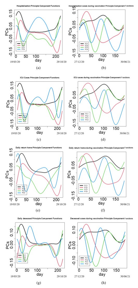
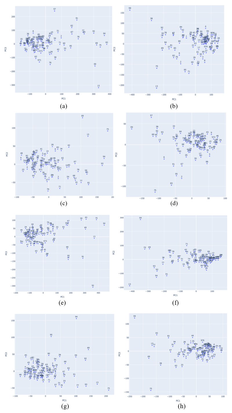
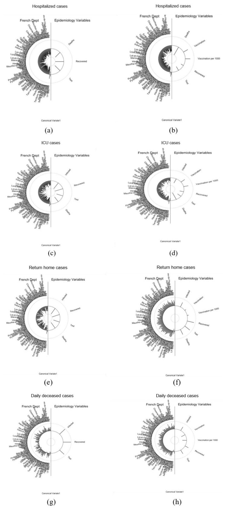
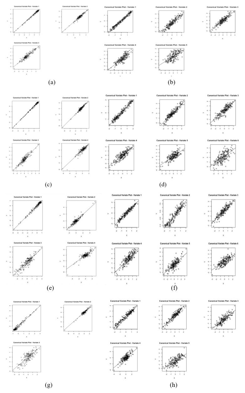
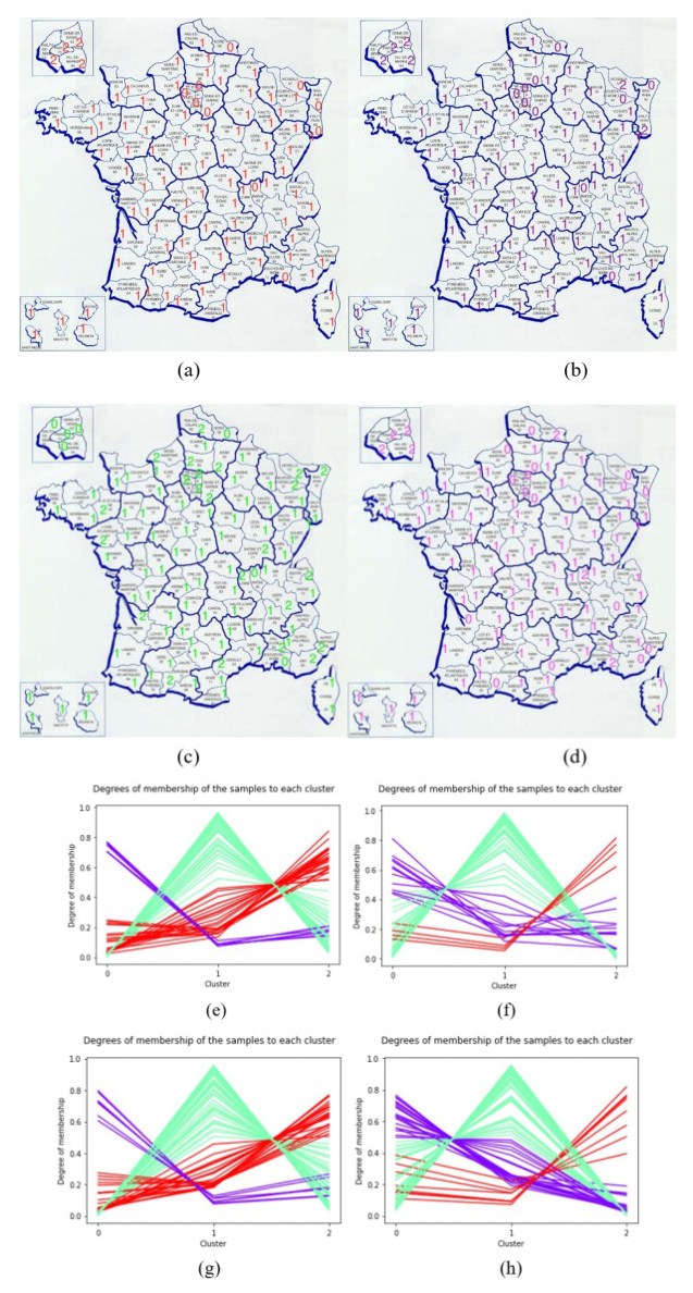
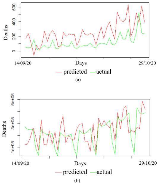
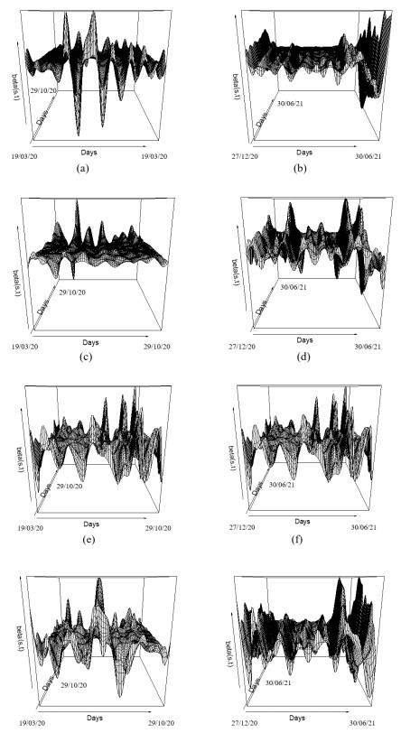
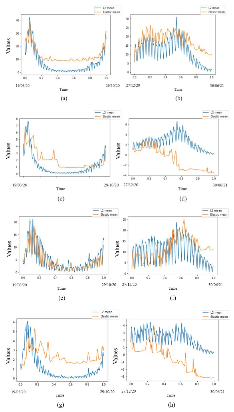
In this paper we use the technique of functional data analysis to model daily hospitalized, deceased, Intensive Care Unit (ICU) cases and return home patient numbers along the COVID-19 outbreak, considered as functional data across different departments in France while our response variables are numbers of vaccinations, deaths, infected, recovered and tests in France. These sets of data were considered before and after vaccination started in France. After smoothing our data set, analysis based on functional principal components method was performed. Then, a clustering using k-means techniques was done to understand the dynamics of the pandemic in different French departments according to their geographical location on France map. We also performed canonical correlations analysis between variables. Finally, we made some predictions to assess the accuracy of the method using functional linear regression models.

Keywords:

canonical correlation,
clustering,
COVID-19,
prediction,
functional data analysis,
functional principal components analysis,
functional linear regression

Citation: Kayode Oshinubi, Firas Ibrahim, Mustapha Rachdi, Jacques Demongeot. Functional data analysis: Application to daily observation of COVID-19 prevalence in France[J]. AIMS Mathematics, 2022, 7(4): 5347-5385. doi: 10.3934/math.2022298

Related Papers:

[1]	Zui-Cha Deng, Fan-Li Liu, Liu Yang . Numerical simulations for initial value inversion problem in a two-dimensional degenerate parabolic equation. AIMS Mathematics, 2021, 6(4): 3080-3104. doi: 10.3934/math.2021187
[2]	Jia Li, Zhipeng Tong . Local Hölder continuity of inverse variation-inequality problem constructed by non-Newtonian polytropic operators in finance. AIMS Mathematics, 2023, 8(12): 28753-28765. doi: 10.3934/math.20231472
[3]	Dun-Gang Li, Fan Yang, Ping Fan, Xiao-Xiao Li, Can-Yun Huang . Landweber iterative regularization method for reconstructing the unknown source of the modified Helmholtz equation. AIMS Mathematics, 2021, 6(9): 10327-10342. doi: 10.3934/math.2021598
[4]	Jia Li, Changchun Bi . Study of weak solutions of variational inequality systems with degenerate parabolic operators and quasilinear terms arising Americian option pricing problems. AIMS Mathematics, 2022, 7(11): 19758-19769. doi: 10.3934/math.20221083
[5]	Yu Xu, Youjun Deng, Dong Wei . Numerical solution of forward and inverse problems of heat conduction in multi-layered media. AIMS Mathematics, 2025, 10(3): 6144-6167. doi: 10.3934/math.2025280
[6]	Zuliang Lu, Fei Cai, Ruixiang Xu, Chunjuan Hou, Xiankui Wu, Yin Yang . A posteriori error estimates of hp spectral element method for parabolic optimal control problems. AIMS Mathematics, 2022, 7(4): 5220-5240. doi: 10.3934/math.2022291
[7]	Batirkhan Turmetov, Valery Karachik . On solvability of some inverse problems for a nonlocal fourth-order parabolic equation with multiple involution. AIMS Mathematics, 2024, 9(3): 6832-6849. doi: 10.3934/math.2024333
[8]	Yashar Mehraliyev, Seriye Allahverdiyeva, Aysel Ramazanova . On one coefficient inverse boundary value problem for a linear pseudoparabolic equation of the fourth order. AIMS Mathematics, 2023, 8(2): 2622-2633. doi: 10.3934/math.2023136
[9]	Guojie Zheng, Baolin Ma . Observability estimate for the parabolic equations with inverse square potential. AIMS Mathematics, 2021, 6(12): 13525-13532. doi: 10.3934/math.2021785
[10]	W. Y. Chan . Blow-up for degenerate nonlinear parabolic problem. AIMS Mathematics, 2019, 4(5): 1488-1498. doi: 10.3934/math.2019.5.1488

Abstract

1. Introduction

The boundary value problems (BVPs) for differential equations have important applications in space science and engineering technology. A large number of mathematical models in the fields of engineering, astronomy, mechanics, economics, etc, are often described by differential BVPs ^[1,2,3]. Except for a few special types, the exact solution of the BVPs is difficult to express in analytical form. It is especially important to find an approximate solution to obtain its numerical solution. In ^[4], Sinc collocation method provided an exponential convergence rate for two-point BVPs. ^[5] constructed a simple collocation method by the Haar wavelets for the numerical solution of linear and nonlinear second-order BVPs with periodic boundary conditions. Erge ^[6] studied the quadratic/linear rational spline collocation method for linear BVPs. In ^[7], based on B-spline wavelets, the numerical solutions of nonlinear BVPs were derived. Pradip et al. used B-spline to Bratuis problem which is an important nonlinear BVPs in ^[8,9,10]. ^{[11,12,13,14,15,16]} solved BVPs by the reproducing kernel method. Based on the idea of least squares, Xu et al. ^[17,18,19] gave an effective algorithm in reproducing kernel space for solving fractional differential integral equations and interface problems.

It is a common technique to use orthogonal polynomials to solve differential equations. In ^{[20,21,22,23]}, the authors used Chebyshev-Galerkin scheme for the time-fractional diffusion equation. In ^[24], the authors developed Jacobi rational operational approach for time-fractional sub-diffusion equation on a semi-infinite domain. ^{[25,26,27,28]} developed multiscale orthonormal basis to solve BVPs with various boundary conditions, and the stability and convergence order were also discussed. Legendre wavelet is widely used in various fields, such as signal system, because of its good properties. In this paper, a multiscale function is constructed by using Legendre polynomials to solve the approximate solution of differential equations. We use the multiscale fine ability of Legendre wavelet to construct multiwavelet, which has better approximation than single wavelet. In addition, we improve Legendre wavelet for specific problems, and the improved one still has compact support. We know that for functions with compact support, the better the tight support, the more concentrated the energy. Moreover, in the calculation process, the calculation speed can be enhanced, and the error accumulation is low.

The purpose of this paper is to construct a set of multiscale orthonormal basis with compact support based on Legendre wavelet to find the approximate solution of the boundary value problems:

$\begin{equation} \left\{ \begin{array}{l} u^{\prime\prime}(x)+p(x)u^{\prime}(x)+q(x)u(x) = F(x, u), \quad x \in (0, 1), \\ a_1u(0)+b_1u(1)+c_1u^{\prime}(0)+d_1u^{\prime}(1) = \alpha_{1}, \\ a_2u(0)+b_2u(1)+c_2u^{\prime}(0)+d_2u^{\prime}(1) = \alpha_{2}, \end{array} \right. \end{equation}$

(1.1)

where $p(x)$ and $q(x)$ are both smooth. $a_i, b_i, c_i, d_i, \; i = 1, 2$ are constants. When $F$ is just about the function of $x$ , $F(x, u) = f(x)$ , Eq (1.1) is linear boundary value problem. According to ^[21], the nonlinear boundary value problem can be transformed into a linear boundary value problem by using Quasi-Newton method. So this paper mainly studies the case of $F(x, u) = f(x)$ , that is, the linear boundary value problem.

As we all know, if the basis function has good properties, the approximate solution of the boundary value problem has good convergence, stability and so on. In ^[25], the orthonormal basis on [0, 1] was constructed by the compact support function to obtain the numerical solution of the boundary value problem. But the basis function is not compactly supported at [0, 1], and the approximating solution is linearly convergent. In this paper, based on the idea of wavelet, a set of orthonormal bases with compact support is constructed by using Legendre polynomials, and the approximate solution of the boundary value problem is obtained by using these bases. Based on the constructed orthonormal basis, the proposed algorithm has convergence and stability, and the convergence order of the algorithm is more than 2 orders.

The purpose of this work is to deduce the numerical solutions of Eq (1.1). In Section 2, using wavelet theory, a set of multiscale orthonormal basis is presented by Legendre polynomials in $W_2^3[0, 1]$ . The constructed basis is compactly supported. It is well known that the compact support performance generates sparse matrices during calculation, thus improving the convergence rate. The numerical method of ${\varepsilon}$ -approximate solution is presented in Section 3. And Section 4 proves the convergence order of ${\varepsilon}$ -approximate solution and stability. In Section 5, the proposed algorithm has been applied to some numerical experiments. Finally, we end with some conclusions in Section 6.

2. Basis functions in $W_2^3[0, 1]$

Wu and Lin introduced the reproducing kernel space $W_2^1[0, 1]$ and $W_2^3[0, 1]$ ^[29]. Let

$W_{2, 0}^3[0, 1] = \{u|u(0) = u^{\prime}(0) = u^{\prime\prime}(0) = 0, \ \ \ u\in W_2^3[0, 1]\}.$

Clearly, $W_{2, 0}^3[0, 1]$ is the closed subspace of $W_2^3[0, 1]$ .

Legendre polynomials are mathematically important functions. This section constructs the orthonormal basis in $W_2^3[0, 1]$ by Legendre polynomials. Legendre polynomials are known to be orthogonal on $L^2[-1, 1]$ . For convenience, we first compress Legendre's polynomials to $[0, 1]$ , and get the following four functions:

$\begin{align*} \varphi^0(x)& = 1; \quad\quad\quad\quad\quad\quad\quad\ \ \varphi^1(x) = \sqrt{3}(-1+2x);\\ \varphi^2(x)& = \sqrt{5}(1-6x+6x^2); \quad \varphi^3(x) = \sqrt{7}(-1+12x-30x^2+20x^3). \end{align*}$

By translating and weighting the above four functions, we can construct

$\begin{equation} \psi^l(x) = \sum\limits_{j = 0}^3(a_{lj}\varphi^j(2x)+b_{lj}\varphi^j(2x-1)), \quad l = 0, 1, 2, 3. \end{equation}$

(2.1)

In application, we hope $\psi^l(x)$ has good properties, for example, as many coefficients as zero and orthogonality, so $\psi^l(x)$ needs to meet the following conditions

$\begin{equation} \int_0^1x^j\psi^l(x)dx = 0, \; \; \; j = 0, 1, 2, \cdots, l+3, \end{equation}$

(2.2)

$\begin{equation} \int_0^1 \psi^i(x)\psi^j(x)dx = \delta_{ij}, \; \; \; i, j = 0, 1, 2, 3. \end{equation}$

(2.3)

The coefficients $a_{lj}, b_{lj}$ can be get by Eqs (2.2) and (2.3), immediately $\psi^l(x)$ is as follows:

$\begin{align} & \psi^0(x) = \sqrt{\frac{15}{17}}\left\{ \begin{array}{l} -3+56x-216x^2+224x^3, \quad x\in [0, \frac{1}{2}], \\ 61-296x+456x^2-224x^3, \quad x\in [\frac{1}{2}, 1]. \end{array} \right. \end{align}$

(2.4)

$\begin{align} &\psi^1(x) = \sqrt{\frac{1}{21}}\left\{ \begin{array}{l} -11+270x-1320x^2+1680x^3, \quad \; \ x\in [0, \frac{1}{2}], \\ -619+2670x-3720x^2+1680x^3, \quad x\in [\frac{1}{2}, 1]. \end{array} \right. \end{align}$

(2.5)

$\begin{align} & \psi^2(x) = \sqrt{\frac{35}{17}}\left\{ \begin{array}{l} -1+30x-174x^2+256x^3, \quad x\in [0, \frac{1}{2}], \\ 111-450x+594x^2-256x^3, \quad x\in [\frac{1}{2}, 1]. \end{array} \right. \end{align}$

(2.6)

$\begin{align} &\psi^3(x) = \sqrt{\frac{5}{21}}\left\{ \begin{array}{l} 1-36x+246x^2-420x^3, \quad x\in [0, \frac{1}{2}], \\ 209-804x+1014x^2-420x^3, \quad x\in [\frac{1}{2}, 1]. \end{array} \right. \end{align}$

(2.7)

Through the ideas of the wavelet, scale transformation of the functions $\psi^l(x)$ gets Legendre wavelet

$\psi^l_{ik}(x) = 2^{\frac{i-1}{2}}\psi^l(2^ix-k), \; \; l = 0, 1, 2, 3;\; \; i = 1, 2, \cdots;\; \; k = 0, 1, \cdots, 2^{i-1}-1.$

Clearly, $\psi_{ik}^{l}(x)$ has compactly support in $[\frac{k}{2^{i-1}}, \frac{k+1}{2^{i-1}}]$ . Let

$W_i = span\{\psi^l_{ik}(x)\}_{l = 0}^3, \; \; i = 1, 2, \cdots;\; \; k = 0, 1, \cdots, 2^{i-1}-1.$

Then,

$L^2[0, 1] = V_0\bigoplus\limits_{i = 1}^{\infty}W_i,$

where

$V_0 = \{\varphi^0(x), \varphi^1(x), \varphi^2(x), \varphi^3(x)\}.$

According to the above analysis, we can get the following theorem.

Theorem 2.1.

$\begin{align*} \begin{aligned} \{\rho_j(x)\}_{j = 1}^{\infty} = \{\varphi^0(x), \varphi^1(x), \varphi^2(x), \varphi^3(x), \psi^0_{10}(x), \psi^1_{10}(x), \psi^2_{10}(x), \psi^3_{10}(x), \cdots, \psi^0_{ik}(x), \psi^1_{ik}(x), \psi^2_{ik}(x), \psi^3_{ik}(x), \cdots \}\end{aligned} \end{align*}$

is the orthonormal basis in $L^2[0, 1]$ .

Now we generate the orthonormal basis in $W_{2, 0}^3[0, 1]$ from the basis in $L^2[0, 1]$ . Note

$\begin{equation} J^{3}u(x) = \frac{1}{2}\int_0^x (x-t)^2u(t)dt. \end{equation}$

(2.8)

Theorem 2.2. $\{J^3\rho_j(x)\}_{j = 1}^{\infty}$ is the orthonormal basis in $W_{2, 0}^3[0, 1]$ .

Proof. Only need to prove completeness and orthogonality. For $u \in W_{2, 0}^3[0, 1]$ , if

$< u, J^3\rho_j > _{W_{2, 0}^3} = 0,$

you can deduce $u \equiv 0$ , then $\{J^3\rho_j(x)\}_{j = 1}^{\infty}$ are complete. In fact,

$\begin{equation} < u, J^3\rho_j > _{W_{2, 0}^3} = < u^{\prime\prime\prime}, \rho_j > _{L^2} = \int_0^1 u^{\prime\prime\prime}\rho_j dx = 0. \end{equation}$

(2.9)

From Theorem 2.1, $u^{\prime\prime\prime}\equiv 0$ . Due to $u \in W_{2, 0}^3[0, 1]$ , $u(0) = u^{\prime}(0) = u^{\prime\prime}(0) = 0$ , then, $u\equiv 0$ .

According to Theorem 2.1 and Eq (2.9), orthonormal is obvious. □

Because of $W^3_{2, 0}[0, 1]\subset W^3_2[0, 1]$ and three more conditions for $W_{2}^3[0, 1]$ than $W_{2, 0}^3[0, 1]$ . So the orthonormal basis for $W_{2}^3[0, 1]$ as follows:

Theorem 2.3.

$\{J^3g_j(x)\}_{j = 1}^{\infty} = \{1, x, \frac{x^2}{2}\} \cup \{J^3\rho_j(x)\}_{j = 1}^{\infty}$

are the orthonormal basis in $W_{2}^3[0, 1]$ .

3. A multiscale algorithm for Eq (1.1)

Put $L$ : $W_2^3[0, 1]\to L^2[0, 1]$ ,

$Lu = u^{\prime\prime}(x)+p(x)u^{\prime}(x)+q(x)u(x).$

$L$ is a linear bounded operator in ^[27]. Let $B_i$ : $W_2^3[0, 1]\to \mathbb{R}$ , and

$B_iu = a_iu(0)+b_iu(1)+c_iu^{\prime}(0)+d_iu^{\prime}(1), \quad i = 1, 2.$

The {Quasi-Newton} method is used to transform Eq (1.1) into a linear boundary value problem, and its operator equation is as follows:

$\begin{equation} \left\{ \begin{array}{l} \quad Lu = f(x), \\ B_1u = \alpha_{1}, \ \ B_2u = \alpha_{2}. \end{array} \right. \end{equation}$

(3.1)

Definition 3.1. $u^{{\varepsilon}}$ is named ${\varepsilon}$ -approximate solution for Eq (3.1), $\forall {\varepsilon} > 0$ , if

$\|Lu^{{\varepsilon}}-f\|_{L^2}^2+\sum\limits_{i = 1}^{2}(B_iu^{{\varepsilon}}-\alpha_i)^2 < {\varepsilon}^2.$

In ^[27], it is shown that ${\varepsilon}$ -approximate solution for Eq (3.1) exists by the following theorem.

Theorem 3.1. Equation (3.1) exists ${\varepsilon}$ -approximate solution

$u_n^{{\varepsilon}}(x) = \sum\limits_{k = 1}^{n} c^{*}_k J^3g_{k}(x) ,$

where $n$ is a natural number determined by ${\varepsilon}$ , and $c^{*}_i$ satisfies

$\|\sum\limits_{k = 1}^{n}c^*_{k}LJ^3g_k -Lu \|_{L^2}^{2}+\sum\limits_{l = 1}^{2}(\sum\limits_{k = 1}^{n}c^*_{k}J^3g_k -B_lu)^2 = \min\limits_{c_k}\{\|\sum\limits_{k = 1}^{n}c_{k}LJ^3g_k -Lu \|_{L^2}^{2}+\sum\limits_{l = 1}^{2}(\sum\limits_{k = 1}^{n}c_{k}J^3g_k -B_lu)^2\}.$

To seek the ${\varepsilon}$ -approximate solution, we just need $c_k^*$ . Let $G$ be quadratic form about

$\mathit{\boldsymbol{c}} = (c_1, \cdots, c_n)^T,$

$\begin{eqnarray} G(c_1, \cdots, c_{n}) = \|\sum\limits_{k = 1}^{n}c_{k}LJ^3g_k -Lu \|_{L^2}^{2}+\sum\limits_{l = 1}^{2}(\sum\limits_{k = 1}^{n}c_{k}J^3g_k -B_lu)^2. \end{eqnarray}$

(3.2)

From Theorem 3.1,

$\mathit{\boldsymbol{c}}^* = (c_1^*, \cdots, c_n^*)^T$

is the minimum point of $G(c_1, \cdots, c_n)$ . If $L$ is reversible, the minimum point of $G$ exists and is unique.

In fact, the partial derivative of $G(c_1, \cdots, c_n)$ with respect to $c_j$ :

$\frac{\partial G}{\partial c_j} = 2 \sum\limits_{k = 1}^{n}c_k\langle LJ^3g_k, LJ^3g_j \rangle_{L^2}-2\langle LJ^3g_j, Lu\rangle_{L^2}+2\sum\limits_{l = 1}^{2}(\sum\limits_{k = 1}^{n}c_kJ^3g_kJ^3g_j-J^3g_jB_lu).$

Let

$\frac{\partial}{\partial c_j}G(c_1, \cdots, c_{n}) = 0,$

$\begin{eqnarray} \sum\limits_{k = 1}^{n}c_k\langle LJ^3g_k, LJ^3g_j \rangle_{L^2}+2\sum\limits_{k = 1}^{n}c_{k}J^3g_k J^3g_j = \langle LJ^3g_j, Lu \rangle_{L^2}+\sum\limits_{l = 1}^{2}J^3g_jB_lu. \end{eqnarray}$

(3.3)

Let $\mathit{\boldsymbol{A_{n}}}$ be the n-order matrix and $\mathit{\boldsymbol{b_{n}}}$ be the n-dimensional vector, i.e.,

$\begin{align*} \begin{array}{c} \mathit{\boldsymbol{A_{n}}} \end{array}& = \left( \begin{array}{c} \langle LJ^3g_k, LJ^3g_j \rangle_{L^2}+2J^3g_k J^3g_j \end{array} \right)_{n\times n}, \\ \begin{array}{c} \mathit{\boldsymbol{b_{n}}} \end{array}& = \left( \begin{array}{c} \langle LJ^3g_k, Lu \rangle_{L^2}+\sum\limits_{l = 1}^{2}J^3g_jB_lu \end{array} \right)_{n}. \end{align*}$

Then Eq (3.3) changes to

$\begin{eqnarray} \mathit{\boldsymbol{A_nc = b_n}}. \end{eqnarray}$

(3.4)

If $L$ is invertible, Eq (3.4) has only one solution $\mathit{\boldsymbol{c}}^*$ , and $\mathit{\boldsymbol{c}}^*$ is minimum point of $G$ . Equation (3.4) has an unique solution is proved as follows.

Theorem 3.2. If $L$ is invertible, Eq (3.3) has only one solution.

Proof. The homogeneous linear equation of Eq (3.4) is

$\begin{eqnarray*} \sum\limits_{k = 1}^{n}c_k\langle LJ^3g_k, LJ^3g_j \rangle_{L^2}+2\sum\limits_{k = 1}^{n}c_{k}J^3g_k J^3g_j = 0. \end{eqnarray*}$

Just prove that the above equation has an unique solution. Let $c_j (j = 1, 2, \cdots, n)$ multiply to both sides of the equation, and add all equations together so that

$\begin{eqnarray*} \langle \sum\limits_{k = 1}^{n}c_k LJ^3g_k, \sum\limits_{j = 1}^{n}c_jLJ^3g_j \rangle_{L^2}+2\sum\limits_{k = 1}^{n}c_{k}J^3g_k \sum\limits_{j = 1}^{n}c_{j}J^3g_j = 0. \end{eqnarray*}$

That is

$\begin{eqnarray*} \|\sum\limits_{k = 1}^{n}c_k LJ^3g_k\|_{L^2}+2(\sum\limits_{k = 1}^{n}c_{k}J^3g_k )^2 = 0. \end{eqnarray*}$

Clearly,

$\|\sum\limits_{k = 1}^{n}c_k LJ^3g_k\|_{L^2}^2 = 0, \qquad (\sum\limits_{k = 1}^{n}c_{k}J^3g_k )^2 = 0.$

Because $J^3g_k$ is orthonormal basis, if $L$ is invertible, $c_k = 0$ . So Eq (3.3) has only one solution. □

4. Analysis of convergence and stability

Convergence and stability are important properties of algorithms. This section deals with the convergence and stability.

4.1. Analysis of convergence

In order to discuss the convergence, Theorem 4.1 is given as follows:

Theorem 4.1. $J^3\psi_{ik}^{l}(x)$ is compactly supported in $[\frac{k}{2^{i-1}}, \frac{k+1}{2^{i-1}}]$ .

Proof. When

$x < \frac{k}{2^{i-1}}, \ \ \ J^3\psi_{ik}^{l}(x) = 0.$

When $x > \frac{k+1}{2^{i-1}}$ , because of $\psi_{ik}^{l}(x)$ with compact support, then,

$\begin{align} J^3\psi_{ik}^{l}(x)& = \frac{1}{2}\int_0^x (x-t)^2\psi_{ik}^{l}(t)dt = \frac{1}{2} \int_{\frac{k}{2^{i-1}}}^{\frac{k+1}{2^{i-1}}}(x-t)^2\psi_{ik}^{l}(t)dt\\ & = 2^{\frac{i-3}{2}} \int_{\frac{k}{2^{i-1}}}^{\frac{k+1}{2^{i-1}}}(x-t)^2\psi^{l}(2^{i-1}t-k)dt\\ & = 2^{-\frac{5(i-1)}{2}} \int_0^1(s-2^{i-1}x-k)^2\psi^{l}(s)ds, \ \; \; s = 2^{i-1}t-k. \end{align}$

(4.1)

According to Eq (2.2), $J^3\psi_{ik}^{l}(x) = 0$ . So $J^3\psi_{ik}^{l}(x)$ has compactly support in $[\frac{k}{2^{i-1}}, \frac{k+1}{2^{i-1}}]$ . □

Note

$(J^3\psi_{i, k}^{l}(x))^{\prime} = J^2\psi_{i, k}^{l}(x), \ \; \; (J^3\psi_{i, k}^{l}(x))^{\prime\prime} = J^1\psi_{i, k}^{l}(x).$

By referring to the proof of Theorem 4.1, $J^1\psi_{ik}^{l}(x)$ and $J^2\psi_{ik}^{l}(x)$ are compactly supported in $[\frac{k}{2^{i-1}}, \frac{k+1}{2^{i-1}}]$ .

The order of convergence will proceed below. Assume

$\begin{equation} u(x) = \sum\limits_{j = 0}^2 c_j\frac{x^j}{j!}+\sum\limits_{j = 0}^3 d_j J^3\varphi^j(x)+\sum\limits_{i = 1}^{\infty}\sum\limits_{k = 0}^{2^{i-1}-1}\sum\limits_{l = 0}^3\left(c_{i, k}^{(l)}J^3\psi_{i, k}^{l}\right), \end{equation}$

(4.2)

where

$c_j = < u, \frac{x^j}{j!} > _{W_2^3}, \ \ \ d_j = < u, \varphi^j(x) > _{W_2^3},$

and

$c_{i, k}^{(l)} = < u, \ \ \ J^3\psi_{i, k}^{l}(x) > _{W_2^3}.$

And

$u_n(x) = \sum\limits_{j = 0}^2 c_j\frac{x^j}{j!}+\sum\limits_{j = 0}^3 d_j J^3\varphi^j(x)+\sum\limits_{i = 1}^{n}\sum\limits_{k = 0}^{2^{i-1}-1}\sum\limits_{l = 0}^3\left(c_{i, k}^{(l)}J^3\psi_{i, k}^{l}\right).$

Theorem 4.2. Assume $u_n^{{\varepsilon}}(x)$ is the ${\varepsilon}$ -approximate solution of Eq (3.1). If $u^{(m)}(x)$ is bounded in $[0, 1]$ , $m \in \mathbb{N}, 3\le m\le7$ , then,

$|u(x)-u_n^{{\varepsilon}}(x)|\le 2^{-(m-2)n}M,$

here $M$ is a constant.

Proof. From Definition 3.1 and Theorem 3.1, we get

$\begin{align} |u(x)-u_n^{{\varepsilon}}(x)|&\le M_0\|u-u_n^{{\varepsilon}}\|_{W_2^3}\le M_0\|L^{-1}\|\|L(u-u_n^{{\varepsilon}})\|_{L^2}\\ &\le M_0\|L^{-1}\|(\|L(u-u_n^{{\varepsilon}})\|_{L^2}+|B_1(u-u_n^{{\varepsilon}})|+|B_2(u-u_n^{{\varepsilon}})|)\\ &\le M_0\|L^{-1}\|(\|L(u-u_n)\|_{L^2}+\|B_1(u-u_n)\|+\|B_2(u-u_n)\|). \end{align}$

Obviously,

$\|B_1(u-u_n)\| = 0, \; \; \; \|B_2(u-u_n)\| = 0.$

That is

$\begin{align} |u(x)-u_n^{{\varepsilon}}(x)| &\le M_0\|L^{-1}\|\|L(u-u_n)\|_{L^2}\le M_0\|L^{-1}\|(\int_0^1 (L(u-u_n))^2dx)^{\frac{1}{2}}\\ &\le M_0\|L^{-1}(\|\max\limits_{x\in [0, 1]}\{|L(u-u_n)|^2\})^{\frac{1}{2}}\\ &\le 3M_0\|L^{-1}\|M_1 \max\limits_{x\in[0, 1]}\{|u-u_n|, |u^{\prime}-u_n^{\prime}|, |u^{\prime\prime}-u_n^{\prime\prime}|\}, \end{align}$

where

$M_1 = \max\limits_{x\in [0, 1]}\{1, |p(x)|, |q(x)|\}.$

We know

$|u-u_n| = |\sum\limits_{i = n+1}^{\infty}\sum\limits_{k = 0}^{2^{i-1}-1}\sum\limits_{l = 0}^{3}c_{i, k}^{(l)}J^3\psi_{i, k}^{l}(x)| \le \sum\limits_{i = n+1}^{\infty}\sum\limits_{k = 0}^{2^{i-1}-1}\sum\limits_{l = 0}^{3}|c_{i, k}^{(l)}||J^3\psi_{i, k}^{l}(x)|.$

By the compactly support of $J^p\psi_{ik}^{l}(x), \; p = 1, 2, 3$ , fixed $i$ , then $J^p\psi_{ik}^{l}(x)\neq 0$ only in $[\frac{k}{2^{i-1}}, \frac{k+1}{2^{i-1}}]$ ,

$|u-u_n| \le \sum\limits_{i = n+1}^{\infty}\sum\limits_{l = 0}^{3}|c_{i, k}^{(l)}||J^3\psi_{i, k}^{l}(x)|.$

Similarly,

$|u^{\prime}-u_n^{\prime}| \le \sum\limits_{i = n+1}^{\infty}\sum\limits_{l = 0}^{3}|c_{i, k}^{(l)}||J^2\psi_{i, k}^{l}(x)|$

and

$|u^{\prime\prime}-u_n^{\prime\prime}| \le \sum\limits_{i = n+1}^{\infty}\sum\limits_{l = 0}^{3}|c_{i, k}^{(l)}||J^1\psi_{i, k}^{l}(x)|.$

Through $J^1\psi_{i, k}^{l}(x), J^2\psi_{i, k}^{l}(x)$ and $J^3\psi_{i, k}^{l}(x)$ , you can get

$|u(x)-u_n^{{\varepsilon}}(x)|\le 3M_0 M_1\|L^{-1}\| |u^{\prime\prime}-u_n^{\prime\prime}|.$

As $|u^{\prime\prime}-u_n^{\prime\prime}|$ , $|c_{i, k}^{(l)}|$ and $|J^1\psi_{i, k}^{l}(x)|$ will be discussed below. We can get that $|c_{i, k}^{(l)}|$ is related to $u^{(m)}(x)$ . In fact,

$\begin{equation} |c_{i, k}^{(l)}| = | < u, J^3\psi_{i, k}^{l}(x) > _{W_2^3}| = |\int_0^1(u^{\prime\prime\prime}(x))\psi_{i, k}^{l}(x)dx| = |\int_{\frac{k}{2^{i-1}}}^{\frac{k+1}{2^{i-1}}}u^{\prime\prime\prime}(x)\psi_{i, k}^{l}(x)dx|. \end{equation}$

(4.3)

Taylor's expansion of $u^{\prime\prime\prime}(x)$ at $\frac{k}{2^{i-1}}$ is

$u^{\prime\prime\prime}(x) = \sum\limits_{j = 3}^{m-1}\frac{u^{(j)}(\frac{k}{2^{i-1}})}{(j-3)!}(x-\frac{k}{2^{i-1}})^{j-3}+\frac{u^{(m)}(\xi)}{(m-3)!}(x-\frac{k}{2^{i-1}})^{m-3}, \ \; \; \; \xi\in[\frac{k}{2^{i-1}}, \frac{k+1}{2^{i-1}}].$

Equation (4.3) is changed to

$\begin{align} |c_{i, k}^{(l)}|& = \left|\int_{\frac{k}{2^{i-1}}}^{\frac{k+1}{2^{i-1}}}\left(\sum\limits_{j = 3}^{m-1}\frac{u^{(j)}(\frac{k}{2^{i-1}})}{(j-3)!}(x-\frac{k}{2^{i-1}})^{j-3}+\frac{u^{(m)}(\xi)}{(m-3)!}(x-\frac{k}{2^{i-1}})^{m-3}\right)\psi_{i, k}^{l}(x)dx\right|\\ & = \left|\sum\limits_{j = 3}^{m-1}\frac{u^{(j)}(\frac{k}{2^{i-1}})}{(j-3)!}\int_{\frac{k}{2^{i-1}}}^{\frac{k+1}{2^{i-1}}}(x-\frac{k}{2^{i-1}})^{j-3}\psi_{ik}^l(x)dx\right|+\left|\int_{\frac{k}{2^{i-1}}}^{\frac{k+1}{2^{i-1}}}\frac{u^{(m)}(\xi)}{(m-3)!}(x-\frac{k}{2^{i-1}})^{m-3})\psi_{i, k}^{l}(x)dx\right|, \end{align}$

where

$\begin{align*} \begin{aligned} \int_{\frac{k}{2^{i-1}}}^{\frac{k+1}{2^{i-1}}}(x-\frac{k}{2^{i-1}})^{j-3}\psi_{ik}^l(x)dx = 2^{\frac{i-1}{2}}\int_{\frac{k}{2^{i-1}}}^{\frac{k+1}{2^{i-1}}}(x-\frac{k}{2^{i-1}})^{j-3}\psi^l(2^{i-1}x-k)dx \mathop = \limits^{t = 2^{i-1}x-k}2^{\frac{(-3-2j)(i-1)}{2}}\int_0^1(t)^{j-3}\psi^l(t)dt.\end{aligned} \end{align*}$

According to Eq (2.2),

$\sum\limits_{j = 3}^{m-1}\frac{u^{(j)}(\frac{k}{2^{i-1}})}{(j-3)!}\int_{\frac{k}{2^{i-1}}}^{\frac{k+1}{2^{i-1}}}(x-\frac{k}{2^{i-1}})^{j-3}\psi_{ik}^l(x)dx = 0,$

$\begin{align} |c_{i, k}^{(l)}|& = \left|\int_{\frac{k}{2^{i-1}}}^{\frac{k+1}{2^{i-1}}}\frac{u^{(m)}(\xi)}{(m-3)!}(x-\frac{k}{2^{i-1}})^{m-3}\psi_{i, k}^{l}(x)dx\right|\\ &\le \left|\frac{u^{(m)}(\xi)}{(m-3)!}\right|\int_{\frac{k}{2^{i-1}}}^{\frac{k+1}{2^{i-1}}}|x-\frac{k}{2^{i-1}}|^{m-3}|\psi_{i, k}^{l}(x)|dx\\ &\le \left|\frac{u^{(m)}(\xi)}{(m-3)!}\right| 2^{-(m-3)(i-1)}\int_{\frac{k}{2^{i-1}}}^{\frac{k+1}{2^{i-1}}}|\psi_{i, k}^{l}(x)|dx\\ &\le \left|\frac{u^{(m)}(\xi)}{(m-3)!}\right| 2^{-(m-3)(i-1)} 2^{-\frac{i-1}{2}}. \end{align}$

Because $u^{(m)}(x)$ is bounded,

$|\frac{u^{(m)}(\xi)}{(m-3)!}|\le M_3,$

then,

$\begin{equation} |c_{i, k}^{(l)}|\le 2^{-\frac{(2m-5)(i-1)}{2}}M_3. \end{equation}$

(4.4)

By the compactly support of $J^1\psi_{ik}^{l}(x)$ ,

$|J^1\psi_{i, k}^{l}(x)| = \left|\int_0^x \psi_{i, k}^{l}(t) dt\right|\le \int_{\frac{k}{2^{i-1}}}^{\frac{k+1}{2^{i-1}}}|\psi_{i, k}^{l}(t)| dt\le 2^{-\frac{i-1}{2}}.$

According to the above analysis,

$|u^{\prime\prime}-u_n^{\prime\prime}|\le\sum\limits_{i = n+1}^{\infty}4M_32^{-\frac{(2m-5)(i-1)}{2}}2^{-\frac{(i-1)}{2}} = 4M_3 2^{-(m-2)n}.$

That is

$|u(x)-u_n^{{\varepsilon}}(x)|\le 2^{-(m-2)n}M,$

where $M$ is a constant. □

4.2. Analysis of stability

Stability analysis is conducted below. According to the third section, the stability of the algorithm is related to the stability of Eq (3.4). By the following Property 4.1, the stability of the algorithm can be discussed by the number of conditions of the matrix $\mathit{\boldsymbol{A}}$ .

Property 4.1. If the matrix $\mathit{\boldsymbol{A}}$ is symmetric and reversible, then

$cond(A) = \bigg|\frac{\lambda_{max}}{\lambda_{min}}\bigg|,$

where ${\lambda_{max}}$ and ${\lambda_{min}}$ are the largest and smallest eigenvalues of $\mathit{\boldsymbol{A}}$ respectively.

In this paper,

$\begin{array}{c} \mathit{\boldsymbol{A_{n}}} \end{array} = \left( \begin{array}{c} a_{ij} \end{array} \right)_{n\times n} = \left( \begin{array}{c} \langle LJ^3g_i, LJ^3g_j \rangle_{L^2}+2J^3g_i J^3g_j \end{array} \right)_{n\times n}.$

Clearly, $\mathit{\boldsymbol{A_{n}}}$ is symmetric. From Theorem 3.2, $\mathit{\boldsymbol{A_{n}}}$ is reversible. In order to discuss the stability of the algorithm, only the eigenvalues of matrix $\mathit{\boldsymbol{A_{n}}}$ need to be discussed.

Theorem 4.3. Assume $u\in W_2^3$ and $\|u\|_{W_2^3} = 1$ . If $L$ is an invertible differential operator, then,

$\|Lu\|_{L^2}\geq \frac{1}{\|L^{-1}\|}.$

Proof. Since $L$ is an invertible, assume $Lu = v$ , then $u = L^{-1}v$ . Moreover

$1 = \|u\|_{W_2^3} = \|L^{-1}v\|_{W_2^3}\leq \|L^{-1}\|\|v\|_{L^2}.$

Then,

$\|v\|_{L^2}\geq \frac{1}{L^{-1}}.$

That is,

$\|Lu\|_{L^2}\geq \frac{1}{\|L^{-1}\|}.$

□

Theorem 4.4. Let ${\lambda}$ {be} the eigenvalues of matrix $\mathit{\boldsymbol{A}}$ of Eq (3.4), $\mathit{\boldsymbol{x}} = (x_1, \cdots, x_n)^{T}$ is related eigenvalue of $\lambda$ and $\|\mathit{\boldsymbol{x}}\| = 1$ , then,

$\lambda\leq \|L\|^2+2.$

Proof. By $\mathit{\boldsymbol{Ax}} = \lambda \mathit{\boldsymbol{x}}$ ,

$\begin{align} \lambda x_i& = \sum\limits_{j = 1}^na_{ij}x_j = \sum\limits_{j = 1}^n(\langle LJ^3g_i, LJ^3g_j \rangle_{L^2}+2J^3g_i J^3g_j)x_j\\ & = \langle LJ^3g_i, \sum\limits_{j = 1}^nx_jLJ^3g_j \rangle_{L^2}+2J^3g_i \sum\limits_{j = 1}^n(J^3g_jx_j), \; \; \; i = 1, \cdots, n. \end{align}$

(4.5)

Let $x_i$ multiply to both sides of Eq (4.5), and then add the equations from $j = 1$ to $j = n$ together so that

$\begin{align} \lambda& = \lambda x_i^2 = \langle \sum\limits_{i = 1}^nx_iLJ^3g_i, \sum\limits_{j = 1}^nx_jLJ^3g_j \rangle_{L^2}+2\sum\limits_{i = 1}^n(J^3g_ix_i)\sum\limits_{j = 1}^n(J^3g_jx_j)\\ & = \big\|\sum\limits_{i = 1}^nx_iLJ^3g_i\big\|_{L^2}^2+2\big(\sum\limits_{i = 1}^n(J^3g_ix_i)\big)^2\\ &\leq \|L\|^2\sum\limits_{i = 1}^nx_i^2+2\sum\limits_{i = 1}^nx_i^2\\ & = (\|L\|^2+2)\|\mathit{\boldsymbol{x}}\|. \end{align}$

(4.6)

Since

$\|\mathit{\boldsymbol{x}}\| = 1, \ \ \ \lambda\leq \|L\|^2+2.$

□

From Theorem 4.3 and Eq (4.6), we can get

$\lambda \geq \big\|\sum\limits_{i = 1}^nx_iLJ^3g_i\big\|_{L^2} = \big\|L(\sum\limits_{i = 1}^nx_iJ^3g_i)\big\|_{L^2}\geq\frac{1}{L^{-1}}.$

Then,

$cond(\mathit{\boldsymbol{A}}) = \big|\frac{\lambda_{max}}{\lambda_{min}}\big|\leq\frac{\|L\|^2+2}{\frac{1}{\|L^{-1}\|}} = (\|L\|^2+2)\|L^{-1}\|.$

That is the condition number of $\mathit{\boldsymbol{A}}$ is bounded, so the presented method is stable.

5. Numerical examples

This section discusses numerical examples to reveal the accuracy of the proposed algorithm. Examples 5.1 and 5.3 are linear and nonlinear BVPs respectively. Example 5.2 shows that our method also applies to Eq (1.1) with other linear boundary value conditions. In this paper, $N$ is the number of bases, and

$N = 7+4*(2^n-1), \; \; \; n = 1, 2, \cdots.$

$e_N(x)$ is the absolute errors. $C.R.$ and $cond$ represent the convergence order and the condition number respectively. For convenience, we denote

$e_N(x) = |u(x)-u_N(x)|$

and

$C.R. = \log_2\frac{\max|e_{N}(x)|}{\max|e_{N+1}(x)|}.$

Example 5.1. Consider the test problem suggested in ^[28,30]

$\begin{equation*} \left\{ \begin{array}{l} u^{\prime\prime} = u^{\prime}+2u+4x-2e^x, \quad x \in (0, 1), \\ u(0) = 2, u(1) = e-1, \end{array} \right. \end{equation*}$

where the exact solution is $u(x) = e^x-2x+1$ . The numerical results are shown in Table 1. It is clear from Table 1 that the present method produces a converging solution for different values. In addition, the results of the proposed algorithm in are compared with those in ^[28,30]. Obviously, the proposed algorithm is better. shows $e_N(x)$ , $C.R.$ , $cond$ and CPU time. The unit of CPU time is second, expressed as $s$ .

Table 1.

$e_N(x)$ of Example 5.1.

$x$	$e_N(x)$ of ^[30]	$e_{66}(x)$ of ^[28]	$e_{35}(x)$	$e_{67}(x)$
$0$	0	5.67e-9	9.94e-14	8.88e-16
$0.1$	1.19e-5	3.35e-9	2.04e-13	2.22e-16
$0.2$	4.18e-5	3.93e-10	2.16e-13	1.55e-15
$0.3$	4.96e-5	1.33e-9	1.42e-13	8.88e-16
$0.4$	6.04e-5	1.40e-9	1.68e-14	1.33e-15
$0.5$	6.33e-5	1.82e-9	1.82e-13	4.44e-16
$0.6$	6.23e-5	5.96e-9	1.52e-13	2.66e-15
$0.7$	5.76e-5	1.14e-8	1.66e-13	8.88e-16
$0.8$	4.23e-5	1.52e-8	4.36e-13	4.44e-15
$0.9$	2.15e-5	1.66e-8	4.93e-13	4.44e-16
$1.0$	0	1.90e-8	2.67e-13	4.44e-15

| Show Table

DownLoad: CSV

Table 2.

$e_N(x)$ ,

$C.R.$ and

$cond$ of Example 5.1.

$n$	$N$	$\max{e_N(x)}$	$C.R.$	$cond$	CPU(s)
$1$	11	1.66e-8		274.262	2.57
$2$	19	6.85e-11	7.92	274.262	7.89
$3$	35	6.55e-13	6.71	274.262	24.42
$4$	67	7.93e-15	6.40	274.262	82.73

| Show Table

DownLoad: CSV

Example 5.2. Consider the problem suggested in ^[25,28].

$\begin{equation*} \left\{ \begin{array}{l} u^{\prime\prime}+u^{\prime}+xu = f(x), \quad x \in (0, 1), \\ u(0) = 2, \quad u(1)+u(\frac{1}{2}) = \sin{\frac{1}{2}}+\sin{1}. \end{array} \right. \end{equation*}$

The exact solution is $u(x) = \sin{x}$ , and $f(x) = \cos{x}-\sin{x}+x\sin{x}$ . This problem is the boundary value problem with the multipoint boundary value conditions. shows maximum absolute error $ME_n$ , $C.R.$ and $cond$ ., which compared with the other algorithms, the results obtained demonstrate that our algorithm is remarkably effective. The numerical errors are provided in Figures 1 and 2, also show a good accuracy.

Table 3.

$ME_n$ , C.R. and

$cond$ of Example 5.2.

The present method				^[25]				^[28]
$n$	$ME_n$	C.R.	$cond$	$n$	$ME_n$	C.R.	$cond$	$n$	$ME_n$	C.R.	$cond$
11	3.73e-9		195.05	10	6.34e-6	3.96	182.06	11	1.88e-4
19	2.97e-11	6.97	195.05	18	4.04e-7	3.98	182.06	19	5.99e-5	1.65	1.49 $\times 10^6$
35	2.13e-13	7.12	195.05	34	2.54e-8	4.06	182.06	35	1.84e-5	1.70	3.74 $\times 10^8$
67	2.77e-15	6.27	195.05	66	1.59e-9	3.95	182.06	67	4.62e-6	1.99	8.87 $\times 10^{10}$

| Show Table

DownLoad: CSV

Figure 1.

$e_N(x)$ of Example 5.3 (n = 35).

DownLoad: Full-Size Img PowerPoint

Figure 2.

$e_N(x)$ of Example 5.3 (n = 67).

DownLoad: Full-Size Img PowerPoint

Example 5.3. Consider a nonlinear problem suggested in ^[7,9]

$\begin{eqnarray*} \left\{ \begin{array}{l} u^{\prime\prime}+\lambda e^{u} = 0, \quad x\in(0, 1)\\ u(0) = 0, u(1) = 0, \end{array} \right. \end{eqnarray*}$

where

$u(x) = -2ln(\cosh((x-\frac{1}{2})(\theta/2))/\cosh(\theta/4)),$

and $\theta$ satisfies

$\theta-\sqrt{2\lambda}\cosh(\theta/4) = 0.$

This is the second-order nonlinear Bratu problem. { Bratu equation is widely used in engineering fields, such as spark discharge, semiconductor manufacturing, etc. In the field of physics, the Bratu equation is used to describe the physical properties of microcrystalline silica gel solar energy. In the biological field, the Bratu equation is used to describe the kinetic model of some biochemical reactions in living organisms.} To this problem, taking $u_0(x) = x(1-x), \; k = 3$ , where $k$ is the number of iterations of the algorithm mentioned in ^[27]. when $\lambda = 1, \lambda = 2$ , $e_N(x)$ are listed in Tables 4 and 5, respectively.

Table 4.

$e_N(x)$ of Example 5.3 (

$\lambda = 1$ ).

$x$	$e_N(x)$ of ^[8]	$e_N(x)$ of ^[9]	$e_N(x)$
0	0	$0$	$4.4959e-11$
0.2	$1.4958e-9$	$2.4390e-5$	$4.1096e-11$
0.4	$2.7218e-9$	$4.2096e-5$	$7.1502e-12$
0.6	$2.7218e-9$	$4.2096e-5$	$7.1483e-12$
0.8	$1.4958e-9$	$2.4390e-5$	$4.1104e-11$

| Show Table

DownLoad: CSV

Table 5.

$e_N(x)$ of Example 5.3 (

$\lambda = 2$ ).

$x$	$e_N(x)$ of ^[7]	$e_N(x)$ of ^[9]	$e_N(x)$
0	$5.8988e-26$	$0$	$1.1801e-12$
0.2	$1.3070e-7$	$6.9297e-5$	$2.5646e-10$
0.4	$1.4681e-7$	$1.0775e-4$	$1.6666e-9$
0.6	$1.4681e-7$	$1.0775e-4$	$1.6666e-9$
0.8	$1.3070e-7$	$6.9297e-5$	$2.5646e-10$

| Show Table

DownLoad: CSV

6. Conclusions

In this paper, based on Legendre's polynomials, we construct orthonormal basis in $L^2[0, 1]$ and $W_2^3[0, 1]$ , respectively. It proves that this group of bases is orthonormal and compactly supported. According to the orthogonality of the basis, we present an algorithm to obtain the approximate solution of the boundary value problems. Using the compact support of the basis, we prove that the convergence order of the presented method related to the boundedness of $u^{(m)}(x)$ . Finally, three numerical examples show that the absolute error and convergence order of the algorithm are better than other methods.

Use of AI tools declaration

The authors declare they have not used Artificial Intelligence (AI) tools in the creation of this article.

Acknowledgments

This study was supported by National Natural Science Funds of China by Grant number (12101164), Characteristic Innovative Scientific Research Project of Guangdong Province (2023KTSCX181, 2023KTSCX183) and Basic and Applied Basic Research Project Zhuhai City (ZH24017003200026PWC).

Conflict of interest

The authors have no conflicts of interest to declare.

References

[1]	D. Bernoulli, Essai d'une nouvelle analyse de la mortalité causée par la petite vérole, et des avantages de l'inoculation pour la prévenir, Histoire de l'Acad., Roy. Sci. (Paris) avec Mem, 1760, 1–45.
[2]	D. A. Henderson, The eradication of smallpox-An overview of the past, present, and future, Vaccine, 29 (2011), D7–D9. https://doi.org/10.1016/j.vaccine.2011.06.080 doi: 10.1016/j.vaccine.2011.06.080
[3]	D. Wujastyk, Medicine in India, In: J. van Alphen, A. Aris, F. Meyer, M. de Fraeye, Oriental medicine: An illustrated guide to the Asian arts of healing, London: Serindia Publications, 1995, 19–38.
[4]	A. M. Silverstein, A history of immunology, 2 Eds., London: Academic Press, 2009,293.
[5]	L. S. Benjamin, L Melville, Lady Mary Wortley Montagu, her life and letters (1689–1762), Hutchinson, London, 1925.
[6]	R. Ross, An application of the theory of probabilities to the study of a priori pathometry-part I, Proc. R. Soc. Ser. A, 92 (1916), 204–230. https://doi.org/10.1098/rspa.1916.0007 doi: 10.1098/rspa.1916.0007
[7]	A. G. McKendrick, Applications of mathematics to medical problems, Proc. Edinburgh Math. Soc., 44 (1925), 98–130. https://doi.org/10.1017/S0013091500034428 doi: 10.1017/S0013091500034428
[8]	J. Gaudart, O. Touré, N. Dessay, A. L. Dicko, S. Ranque, L. Forest, et al., Modelling malaria incidence with environmental dependency in a locality of Sudanese savannah area, Mali. Malaria J., 8 (2009), 61. https://doi.org/10.1186/1475-2875-8-61 doi: 10.1186/1475-2875-8-61
[9]	J. Gaudart, M. Ghassani, J. Mintsa, M. Rachdi, J. Waku, J. Demongeot, Demography and diffusion in epidemics: Malaria and black death spread, Acta Biotheor., 58 (2010), 277–305. https://doi.org/10.1007/s10441-010-9103-z doi: 10.1007/s10441-010-9103-z
[10]	J. Demongeot, J. Gaudart, A. Lontos, E. Promayon, J. Mintsa, M. Rachdi, Zero-diffusion domains in reaction-diffusion morphogenetic and epidemiologic processes, Int. J. Bifurcation Chaos, 22 (2012), 1250028. https://doi.org/10.1142/S0218127412500289 doi: 10.1142/S0218127412500289
[11]	J. Demongeot, J. Gaudart, J. Mintsa, M. Rachdi, Demography in epidemics modelling, Commun. Pure Appl. Anal., 11 (2012), 61–82. http://dx.doi.org/10.3934/cpaa.2012.11.61 doi: 10.3934/cpaa.2012.11.61
[12]	Z. Liu, P. Magal, O. Seydi, G. Webb, Understanding unreported cases in the COVID-19 epidemic outbreak in Wuhan, China, and importance of major public health interventions, Biology, 9(2020), 50. https://doi.org/10.3390/biology9030050 doi: 10.3390/biology9030050
[13]	J. Demongeot, Q. Griette, P. Magal, SI epidemic model applied to COVID-19 data in mainland China, Royal Soc. Open Sci., 7 (2020), 201878. https://doi.org/10.1098/rsos.201878 doi: 10.1098/rsos.201878
[14]	Z. Liu, P. Magal, O. Seydi, G. Webb, Predicting the cumulative number of cases for the COVID-19 epidemic in China from early data, Math. Biosci. Eng., 17 (2020), 3040–3051. https://doi.org/10.3934/mbe.2020172 doi: 10.3934/mbe.2020172
[15]	P. Magal, O. Seydi, G. Webb, Y. Wu, A model of vaccination for Dengue in the Philippines 2016–2018, Front. Appl. Math. Stat., 7 (2021), 760259. https://doi.org/10.3389/fams.2021.760259 doi: 10.3389/fams.2021.760259
[16]	K. Oshinubi, M. Rachdi, J. Demongeot, Modelling of COVID-19 pandemic vis-à-vis some socioeconomic factors, Front. Appl. Math. Stat., 7 (2021), 786983.
[17]	COVID-19 coronavirus pandemic, 2021. Available from: https://www.worldometers.info/coronavirus.
[18]	Données hospitalières relatives à l'épidémie de COVID-19, 2021. Available from: https://www.data.gouv.fr/fr/datasets/donnees-hospitalieres-relatives-a-lepidemie-de-Covid-19.
[19]	Live COVID-19 vaccination tracker. Available from: https://covidvax.live/location/fra.
[20]	F. Ferraty, P. Vieu, Nonparametric functional data analysis, New York: Springer, 2006. https://doi.org/10.1007/0-387-36620-2
[21]	J. D. Tucker, Functional component analysis and regression using elastic methods, PhD. Thesis, Florida State University, 2014.
[22]	J. D. Tucker, W. Wu, A. Srivastava, Generative models for functional data using phase and amplitude separation, Comput. Stat. Data Anal., 61 (2013), 50–66. https://doi.org/10.1016/j.csda.2012.12.001 doi: 10.1016/j.csda.2012.12.001
[23]	J. O. Ramsay, B. W. Silverman, Applied functional data analysis: Methods and case studies, New York: Springer, 2002. https://doi.org/10.1007/b98886
[24]	A. Srivastava, E. P. Klassen, Functional data and elastic registration, In: Functional and shape data analysis, New York: Springer, 2016, 73–123. https://doi.org/10.1007/978-1-4939-4020-2_4
[25]	J. O. Ramsay, G. Hooker, S. Graves, Functional data analysis with R and MATLAB, New York: Springer, 2009. https://doi.org/10.1007/978-0-387-98185-7
[26]	C. Tang, T. Wang, P. Zhang, Functional data analysis: An application to COVID-19 data in the United States, arXiv. Available from: https://arXiv.org/abs/2009.08363.
[27]	C. Acal, M. Escabias, A. M. Aguilera, M. J. Valderrama, COVID-19 data imputation by multiple function-on-function principal component regression, Mathematics, 9 (2021), 1237. https://doi.org/10.3390/math9111237 doi: 10.3390/math9111237
[28]	T. Boschi, J. Di Iorio, L. Testa, M. A. Cremona, F. Chiaromonte, Functional data analysis characterizes the shapes of the first COVID-19 epidemic wave in Italy, Sci. Rep., 11 (2021), 17054. https://doi.org/10.1038/s41598-021-95866-y doi: 10.1038/s41598-021-95866-y
[29]	Q. Griette, J. Demongeot, P. Magal, A robust phenomenological approach to investigate COVID-19 data for France, Math. Appl. Sci. Eng., 2 (2021), 149–218. https://doi.org/10.5206/mase/14031 doi: 10.5206/mase/14031
[30]	Q. Griette, J. Demongeot, P. Magal, What can we learn from COVID-19 data by using epidemic models with unidentied infectious cases, Math. Biosci. Eng., 2 (2021), 149–160. http://dx.doi.org/10.2139/ssrn.3868852 doi: 10.2139/ssrn.3868852
[31]	J. Gaudart, J. Landier, L. Huiart, E. Legendre, L. Lehot, M. K. Bendiane, et al., Factors associated with spatial heterogeneity of Covid-19 in France: A nationwide ecological study, Lancet Public Health, 6(2021), 222–231. https://doi.org/10.1016/s2468-2667(21)00006-2 doi: 10.1016/S2468-2667(21)00006-2
[32]	O. D. Ilie, R. O. Cojocariu, A. Ciobica, S. I. Timofte, I. Mavroudis, B. Doroftei, Forecasting the spreading of COVID-19 across nine countries from Europe, Asia, and the American continents using the ARIMA models, Microorganisms, 8 (2020), 1158. https://doi.org/10.3390/microorganisms8081158 doi: 10.3390/microorganisms8081158
[33]	J. Stojanovic, V. G. Boucher, J. Boyle, J. Enticott, K. L. Lavoie, S. L. Bacon, COVID-19 is not the flu: Four graphs from four countries, Front. Public Health, 2021, 628479. https://doi.org/10.3389/fpubh.2021.628479 doi: 10.3389/fpubh.2021.628479
[34]	C. Carroll, S. Bhattacharjee, Y. Chen, P. Dubey, J. Fan, A. Gajardo, et al., Time dynamics of COVID-19, Sci. Rep., 10 (2020), 21040. https://doi.org/10.1038/s41598-020-77709-4 doi: 10.1038/s41598-020-77709-4
[35]	A. Srivastava, G. Chowell, Modeling study: Characterizing the spatial heterogeneity of the COVID-19 pandemic through shape analysis of epidemic curves, Res. Square, 2021, 1–27. https://doi.org/10.21203/rs.3.rs-223226/v1 doi: 10.21203/rs.3.rs-223226/v1
[36]	J. Demongeot, Y. Flet-Berliac, H. Seligmann, Temperature decreases spread parameters of the new COVID-19 cases dynamics, Biology, 9 (2020), 94. https://doi.org/10.3390/biology9050094 doi: 10.3390/biology9050094
[37]	H. Seligmann, S. Iggui, M. Rachdi, N. Vuillerme, J. Demongeot, Inverted covariate effects for mutated 2^nd vs 1^st wave COVID-19: High temperature spread biased for young, Biology, 9 (2020), 226. https://doi.org/10.1101/2020.07.12.20151878 doi: 10.3390/biology9080226
[38]	S. Soubeyrand, J. Demongeot, L. Roques, Towards unified and real-time analyses of outbreaks at country-level during pandemics, One Health, 11 (2020), 100187. https://doi.org/10.1016/j.onehlt.2020.100187 doi: 10.1016/j.onehlt.2020.100187
[39]	J. Demongeot, H. Seligmann, SARS-CoV-2 and miRNA-like inhibition power, Med. Hypotheses, 144 (2020), 110245. https://doi.org/10.1016/j.mehy.2020.110245 doi: 10.1016/j.mehy.2020.110245
[40]	H. Seligmann, N. Vuillerme, J. Demongeot, Unpredictable, counter-intuitive geoclimatic and demographic correlations of COVID-19 spread rates, Biology, 10 (2021), 623. https://doi.org/10.3390/biology10070623 doi: 10.3390/biology10070623
[41]	K. Oshinubi, F. Al-Awadhi, M. Rachdi, J. Demongeot, Data analysis and forecasting of COVID-19 pandemic in Kuwait, MedRxiv, 2021, 1–17. https://doi.org/10.1101/2021.07.24.21261059 doi: 10.1101/2021.07.24.21261059
[42]	J. Demongeot, K. Oshinubi, M. Rachdi, L. Hobbad, M. Alahiane, S. Iggui, et al., The application of ARIMA model to analyze COVID-19 incidence pattern in several countries, J. Math. Comput. Sci., 12 (2022), 1–23. https://doi.org/10.28919/jmcs/6541 doi: 10.28919/jmcs/6541
[43]	K. Oshinubi, M. Rachdi, J. Demongeot, Analysis of reproduction number R₀ of COVID-19 using current health expenditure as gross domestic product percentage (CHE/GDP) across countries, Healthcare, 9 (2021), 1247. https://doi.org/10.3390/healthcare9101247 doi: 10.3390/healthcare9101247
[44]	J. Demongeot, K. Oshinubi, M. Rachdi, H. Seligmann, F. Thuderoz, J. Waku, Estimation of daily reproduction rates in COVID-19 outbreak, MedRxiv, 9 (2021), 109. https://doi.org/10.1101/2020.12.30.20249010 doi: 10.1101/2020.12.30.20249010
[45]	J. Demongeot, A. Laksaci, F. Madani, M. Rachdi, Functional data: Local linear estimation of the conditional density and its application, Statistics, 47 (2013), 26–44. https://doi.org/10.1080/02331888.2011.568117 doi: 10.1080/02331888.2011.568117
[46]	M. Rachdi, A. Laksaci, J. Demongeot, A. Abdali, F. Madani, Theoretical and practical aspects on the quadratic error in the local linear estimation of the conditional density for functional data, Comput. Stat. Data Anal., 73 (2014), 53–68. https://doi.org/10.1016/j.csda.2013.11.011 doi: 10.1016/j.csda.2013.11.011
[47]	J. Demongeot, A. Laksaci, M. Rachdi, S. Rahmani, On the local linear modelization of the conditional distribution for functional data, Sankhya A, 76 (2014), 328–355. https://doi.org/10.1007/s13171-013-0050-z doi: 10.1007/s13171-013-0050-z
[48]	J. Demongeot, A. Hamie, A. Laksaci, M. Rachdi, Relative-error prediction in nonparametric functional statistics: Theory and practice, J. Multivar. Anal., 146 (2016), 261–268. https://doi.org/10.1016/j.jmva.2015.09.019 doi: 10.1016/j.jmva.2015.09.019
[49]	J. Demongeot, A. Laksaci, A. Naceri, M. Rachdi, Local linear regression modelization when all variables are curves, Stat. Probab. Lett., 121 (2017), 37–44. https://doi.org/10.1016/j.spl.2016.09.021 doi: 10.1016/j.spl.2016.09.021
[50]	A. Belkis, J. Demongeot, A. Laksaci, M. Rachdi, Functional data analysis: Estimation of the relative error in functional regression under random left-truncation, J. Nonparametr. Stat., 30 (2018), 472–490. https://doi.org/10.1080/10485252.2018.1438609 doi: 10.1080/10485252.2018.1438609
[51]	A. Henien, L. Ait-Hennani, J. Demongeot, A. Laksaci, M. Rachdi, Heteroscedasticity test when the covariables are functionals, C. R. Math., 356 (2018), 571–574. https://doi.org/10.1016/j.crma.2018.02.010 doi: 10.1016/j.crma.2018.02.010
[52]	J. Demongeot, O. Hansen, H. Hessami, A. S. Jannot, J. Mintsa, M. Rachdi, et al., Random modelling of contagious diseases, Acta Biotheor., 61 (2013), 141–172. https://doi.org/10.1007/s10441-013-9176-6 doi: 10.1007/s10441-013-9176-6
[53]	C. J. Rhodes, L. Demetrius, Evolutionary entropy determines invasion success in emergent epidemics, PLoS One, 5 (2010), e12951. https://doi.org/10.1371/journal.pone.0012951 doi: 10.1371/journal.pone.0012951
[54]	S. Triambak, D. P. Mahapatra, A random walk Monte Carlo simulation study of COVID-19-like infection spread, Physica A: Stat. Mech. Appl., 574 (2021), 126014. https://doi.org/10.1016/j.physa.2021.126014 doi: 10.1016/j.physa.2021.126014
[55]	Wikipedia, Available online: https://www.wikipedia.org/wiki/Departments_of_France.

This article has been cited by:

1.	Mohammed Elamine Beroudj, Abdelaziz Mennouni, Carlo Cattani, Hermite solution for a new fractional inverse differential problem, 2024, 0170-4214, 10.1002/mma.10516
2.	苗苗宋, Inverse Problem of Option Drift Rate Based on Degenerate Parabolic Equations, 2023, 12, 2324-7991, 3814, 10.12677/AAM.2023.129375
3.	Yilihamujiang Yimamu, Zui-Cha Deng, C. N. Sam, Y. C. Hon, Total variation regularization analysis for inverse volatility option pricing problem, 2024, 101, 0020-7160, 483, 10.1080/00207160.2024.2345660

Reader Comments

Your name:*

Email:*
© 2022 the Author(s), licensee AIMS Press. This is an open access article distributed under the terms of the Creative Commons Attribution License (http://creativecommons.org/licenses/by/4.0)