Upper paired domination in graphs

Huiqin Jiang; Pu Wu; Jingzhong Zhang; Yongsheng Rao; Huiqin Jiang; Pu Wu; Jingzhong Zhang; Yongsheng Rao

doi:10.3934/math.2022069

AIMS Mathematics

2022, Volume 7, Issue 1: 1185-1197. doi: 10.3934/math.2022069

Previous Article Next Article

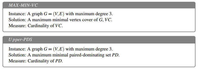
Research article

Upper paired domination in graphs

1.
Institute of Computing Science and Technology, Guangzhou University, Guangzhou 510006, China
2.
School of Electronics Engineering and Computer Science, Peking University, Beijing 100871, China

Received: 23 May 2021 Accepted: 29 September 2021 Published: 21 October 2021
MSC : 05C69, 68Q15

A set $ PD\subseteq V(G) $ in a graph $ G $ is a paired dominating set if every vertex $ v\notin PD $ is adjacent to a vertex in $ PD $ and the subgraph induced by $ PD $ contains a perfect matching. A paired dominating set $ PD $ of $ G $ is minimal if there is no proper subset $ PD'\subset PD $ which is a paired dominating set of $ G $. A minimal paired dominating set of maximum cardinality is called an upper paired dominating set, denoted by $ \Gamma_{pr}(G) $-set. Denote by $ Upper $-$ PDS $ the problem of computing a $ \Gamma_{pr}(G) $-set for a given graph $ G $. Michael et al. showed the APX-completeness of $ Upper $-$ PDS $ for bipartite graphs with $ \Delta = 4 $ ^[11]. In this paper, we show that $ Upper $-$ PDS $ is APX-complete for bipartite graphs with $ \Delta = 3 $.
- upper paired domination,
- APX-completeness
Citation: Huiqin Jiang, Pu Wu, Jingzhong Zhang, Yongsheng Rao. Upper paired domination in graphs[J]. AIMS Mathematics, 2022, 7(1): 1185-1197. doi: 10.3934/math.2022069

Related Papers:

Abstract

A set $ PD\subseteq V(G) $ in a graph $ G $ is a paired dominating set if every vertex $ v\notin PD $ is adjacent to a vertex in $ PD $ and the subgraph induced by $ PD $ contains a perfect matching. A paired dominating set $ PD $ of $ G $ is minimal if there is no proper subset $ PD'\subset PD $ which is a paired dominating set of $ G $. A minimal paired dominating set of maximum cardinality is called an upper paired dominating set, denoted by $ \Gamma_{pr}(G) $-set. Denote by $ Upper $-$ PDS $ the problem of computing a $ \Gamma_{pr}(G) $-set for a given graph $ G $. Michael et al. showed the APX-completeness of $ Upper $-$ PDS $ for bipartite graphs with $ \Delta = 4 $ ^[11]. In this paper, we show that $ Upper $-$ PDS $ is APX-complete for bipartite graphs with $ \Delta = 3 $.

References

[1]	G. Ausiello, M. Protasi, A. Marchettispaccamela, G. Gambosi, P. Crescenzi, V. Kann, Complexity and Approximation: Combinatorial Optimization Problems and Their Approximability Properties, Springer-Verlag, Berlin, 1999.
[2]	C. Bazgan, L. Brankovic, K. Casel, H. Fernau, On the complexity landscape of the domination chain, In: Proceedings of the Second International Conference on Algorithms and Discrete Applied Mathematics, 2016, 61–72.
[3]	J. A. Bondy, U. S. R. Murty, Graph theory with applications, USA, 1976.
[4]	L. Chen, C. Lu, Z. Zeng, Labelling algorithms for paired-domination problems in block and interval graphs, J. Comb. Optim., 19 (2010), 457–470. doi: 10.1007/s10878-008-9177-6. doi: 10.1007/s10878-008-9177-6
[5]	E. J. Cockayne, O. Favaron, C. M. Mynhardt, Paired-domination in claw-free cubic graphs, Graphs Combinatorics, 20 (2004), 447–456. doi: 10.1007/s00373-004-0577-9. doi: 10.1007/s00373-004-0577-9
[6]	P. Dorbec, S. Gravier, M. A. Henning, Paired-domination in generalized claw-free graphs, J. Comb. Optim., 14 (2007), 1–7. doi: 10.1007/s10878-006-9022-8. doi: 10.1007/s10878-006-9022-8
[7]	P. Dorbec, M. A. Henning, J. Mccoy, Upper total domination versus upper paired-domination, Quaestiones Mathematicae, 30 (2007), 1–12. doi: 10.2989/160736007780205693. doi: 10.2989/160736007780205693
[8]	M. R. Garey, D. S. Johnson, Computers and intractability: A guide to the theory of NP-completeness, WH Freeman & Co., New York, 1979.
[9]	T. W. Haynes, P. J. Slater, Paired-domination in graphs, Networks, 32 (1998), 199–206. doi: 10.1002/(SICI)1097-0037(199810)32:3<199::AID-NET4>3.0.CO;2-F. doi: 10.1002/(SICI)1097-0037(199810)32:3<199::AID-NET4>3.0.CO;2-F
[10]	M. A. Henning, P. Dorbec, Upper paired-domination in claw-free graphs, J. Comb. Optim., 22 (2011), 235–251. doi: 10.1007/s10878-009-9275-0. doi: 10.1007/s10878-009-9275-0
[11]	M. A. Henning, D. Pradhan, Algorithmic aspects of upper paired-domination in graphs, Theor. Comput. Sci., 804 (2020), 98–114. doi: 10.1016/j.tcs.2019.10.045. doi: 10.1016/j.tcs.2019.10.045
[12]	C. Lu, B. Wang, K. Wang, Y. Wu, Paired-domination in claw-free graphs with minimum degree at least three, Discrete Appl. Math., 257 (2019), 250–259. doi: 10.1016/j.dam.2018.09.005. doi: 10.1016/j.dam.2018.09.005
[13]	S. Mishra, K. Sikdar, On the hardness of approximating some NP-optimization problems related to minimum linear ordering problem, Rairo-Theor. Inf. Appl., 35 (2001), 287–309. doi: 10.1051/ita:2001121. doi: 10.1051/ita:2001121
[14]	A. Pandey, B. S. Panda, Domination in some subclasses of bipartite graphs, Discrete Appl. Math., 252 (2015), 169–180. doi: 10.1007/978-3-319-14974-5_17. doi: 10.1007/978-3-319-14974-5_17
[15]	C. H. Papadimitriou, M. Yannakakis, Optimization, approximation, and complexity classes, J. Comput. Syst. Sci., 43 (1991), 425–440. doi: 10.1016/0022-0000(91)90023-X. doi: 10.1016/0022-0000(91)90023-X
[16]	D. Pradhan, B. S. Panda, Computing a minimum paired-dominating set in strongly orderable graphs, Discrete Appl. Math., 253 (2018), 37–50. doi: 10.1016/j.dam.2018.08.022. doi: 10.1016/j.dam.2018.08.022
[17]	H. Qiao, L. Kang, M. Cardei, D. Du, Paired-domination of trees, J. Global Optim., 25 (2003), 43–54. doi: 10.1023/A:1021338214295. doi: 10.1023/A:1021338214295
[18]	D. B. West, Introduction to graph theory, 2nd ed., Prentice Hall, USA, 2001.

Reader Comments

Your name:*

Email:*
© 2022 the Author(s), licensee AIMS Press. This is an open access article distributed under the terms of the Creative Commons Attribution License (http://creativecommons.org/licenses/by/4.0)