Two linearized finite difference schemes for time fractional nonlinear diffusion-wave equations with fourth order derivative

Emadidin Gahalla Mohmed Elmahdi; Jianfei Huang; Emadidin Gahalla Mohmed Elmahdi; Jianfei Huang

doi:10.3934/math.2021373

AIMS Mathematics

2021, Volume 6, Issue 6: 6356-6376. doi: 10.3934/math.2021373

Previous Article Next Article

Research article

Two linearized finite difference schemes for time fractional nonlinear diffusion-wave equations with fourth order derivative

Emadidin Gahalla Mohmed Elmahdi ^1,2,
Jianfei Huang ^{1
,
,}

1.
College of Mathematical Sciences, Yangzhou University, Yangzhou 225002, China
2.
Faculty of Education, University of Khartoum, Khartoum P. O. Box 321, Sudan

Received: 25 January 2021 Accepted: 08 April 2021 Published: 12 April 2021
MSC : 65M06, 65M12

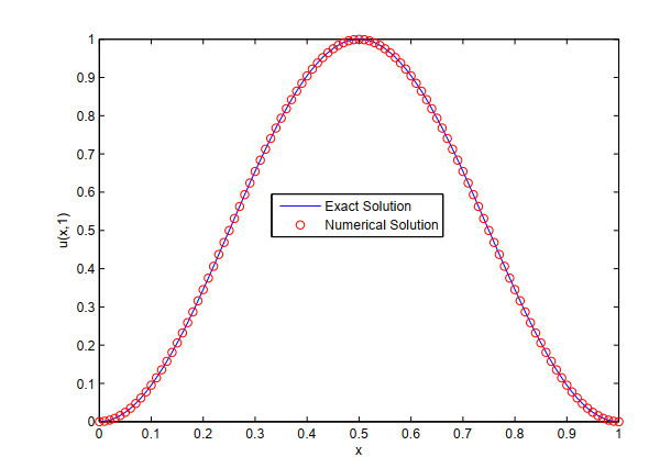
In this paper, we present a linearized finite difference scheme and a compact finite difference scheme for the time fractional nonlinear diffusion-wave equations with space fourth order derivative based on their equivalent partial integro-differential equations. The finite difference scheme is constructed by using the Crank-Nicolson method combined with the midpoint formula, the weighted and shifted Gr$ \ddot{\text{u}} $nwald difference formula and the second order convolution quadrature formula to deal with the temporal discretizations. Meanwhile, the classical central difference formula and fourth order Stephenson scheme are used in the spatial direction. Then, the compact finite difference scheme is developed by using the fourth order compact difference formula for the spatial direction. The proposed schemes can deal with the nonlinear terms in a flexible way while meeting weak smoothness requirements in time. Under the relatively weak smoothness conditions, the stability and convergence of the proposed schemes are strictly proved by using the discrete energy method. Finally, some numerical experiments are presented to support our theoretical results.
- fractional nonlinear diffusion-wave equations,
- linearized schemes,
- fourth order derivative,
- stability,
- convergence
Citation: Emadidin Gahalla Mohmed Elmahdi, Jianfei Huang. Two linearized finite difference schemes for time fractional nonlinear diffusion-wave equations with fourth order derivative[J]. AIMS Mathematics, 2021, 6(6): 6356-6376. doi: 10.3934/math.2021373

Related Papers:

Abstract

In this paper, we present a linearized finite difference scheme and a compact finite difference scheme for the time fractional nonlinear diffusion-wave equations with space fourth order derivative based on their equivalent partial integro-differential equations. The finite difference scheme is constructed by using the Crank-Nicolson method combined with the midpoint formula, the weighted and shifted Gr$ \ddot{\text{u}} $nwald difference formula and the second order convolution quadrature formula to deal with the temporal discretizations. Meanwhile, the classical central difference formula and fourth order Stephenson scheme are used in the spatial direction. Then, the compact finite difference scheme is developed by using the fourth order compact difference formula for the spatial direction. The proposed schemes can deal with the nonlinear terms in a flexible way while meeting weak smoothness requirements in time. Under the relatively weak smoothness conditions, the stability and convergence of the proposed schemes are strictly proved by using the discrete energy method. Finally, some numerical experiments are presented to support our theoretical results.

References

[1]	R. Herrmann, Fractional Calculus, An Introduction for Physicists ($2^{nd}$ Edition), Singapore, World Scientific, 2014.
[2]	D. Baleanu, O. Defterli, O. P. Agrawal, A central difference numerical scheme for fractional optimal control problems, J. Vib. Control., 15 (2009), 583–597. doi: 10.1177/1077546308088565
[3]	T. S. Aleroev, H. T. Aleroeva, J. F. Huang, N. M. Nie, Y. F. Tang, et al., Features of seepage of a liquid to a chink in the cracked deformable layer, Int. J. Model. Simul. Sci. Comput., 1 (2010), 333–347. doi: 10.1142/S1793962310000195
[4]	L. Song, W. Wang, Solution of the fractional Black-Scholes option pricing model by finite difference method, Abstr. Appl. Anal., 45 (2013), 1–16.
[5]	R. Metzler, J. Klafter, Boundary value problems for fractional diffusion equations, Physica A., 278 (2000), 107–125. doi: 10.1016/S0378-4371(99)00503-8
[6]	W. R. Schneider, W. Wyss, Fractional diffusion and wave equations, J. Math. Phys., 30 (1989), 134–144. doi: 10.1063/1.528578
[7]	Y. Luchko, F. Mainardi, Some properties of the fundamental solution to the signalling problem for the fractional diffusion-wave equation, Cent. Eur. J. Phys., 11 (2013), 666–675.
[8]	X. Hu, L. Zhang, On finite difference methods for fourth-order fractional diffusion-wave and sub-diffusion systems, Appl. Math. Comput., 218 (2012), 5019–5034. doi: 10.1016/j.amc.2011.10.069
[9]	J. F. Huang, D. D. Yang, A unified difference-spectral method for time-space fractional diffusion equations, Int. J. Comput. Math., 94 (2017), 1172–1184. doi: 10.1080/00207160.2016.1184262
[10]	O. Nikan, A. Golbabai, J. T. Machado, T. Nikazad, Numerical approximation of the time fractional cable equation arising in neuronal dynamics, Eng. Comput., (2020), 1–19.
[11]	F. Zeng, Second order stable finite difference schemes for the time fractional diffusion-wave equation, J. Sci. Comput., 65 (2015), 411–430. doi: 10.1007/s10915-014-9966-2
[12]	O. Nikan, H. Jafari, A. Golbabai, Numerical analysis of the fractional evolution model for heat flow in materials with memory, Alexandria Eng. J., 59 (2020), 2627–2637. doi: 10.1016/j.aej.2020.04.026
[13]	R. R. Nigmatullin, To the theoretical explanation of the universal response, Phys. Status Solidi, B Basic Res., 123 (1984), 739–745.
[14]	R. R. Nigmatullin, Realization of the generalized transfer equation in a medium with fractal geometry, Phys. Status Solidi, B Basic Res., 133 (1986), 425–430. doi: 10.1002/pssb.2221330150
[15]	K. B. Oldham, J. Spanier, The Fractional Calculus, Academic Press, NewYork, 1974.
[16]	A. H. Bhrawy, E. H. Doha, D. Baleanud, S. S. Ezz-Eldien, A spectral tau algorithm based on Jacobi operational matrix for numerical solution of time fractional diffusion-wave equations, J. Comput. Phys., 293 (2015), 142–156. doi: 10.1016/j.jcp.2014.03.039
[17]	J. Chen, F. Liu, V. Anh, S. Shen, Q. Liu, et al., The analytical solution and numerical solution of the fractional diffusion-wave equation with damping, Appl. Math. Comput., 219 (2012), 1737–1748. doi: 10.1016/j.amc.2012.08.014
[18]	A. Ebadian, H. R. Fazli, A. A. Khajehnasiri, Solution of nonlinear fractional diffusion-wave equation by traingular functions, SeMA. J., 72 (2015), 37–46. doi: 10.1007/s40324-015-0045-x
[19]	M. H. Heydari, M. R. Hooshmandasl, F. M. Maalek Ghaini, C. Cattani, Wavelets method for the time fractional diffusion-wave equation, Phys. Lett. A., 379 (2015), 71–76. doi: 10.1016/j.physleta.2014.11.012
[20]	N. Khalid, M. Abbas, M. K. Iqbal, D. Baleanu, A numerical algorithm based on modified extended b-spline functions for solving time-fractional diffusion wave equation involving reaction and damping terms, Adv. Differ. Equ., 2019 (2019), 378. doi: 10.1186/s13662-019-2318-7
[21]	O. H. Mohammed, S. F. Fadhel, M. G. S. AL-Safi, Numerical solution for the time fractional diffusion-wave equations by using Sinc-Legendre collocation method, Math. Theory. Model., 5 (2015), 49–57.
[22]	F. Y. Zhou, X. Y. Xu, Numerical solution of time-fractional diffusion-wave equations via Chebyshev wavelets collocation method, Adv. Math. Phys., 2017 (2017), 2610804.
[23]	H. Y. He, K. J. Liang, B. L. Yin, A numerical method for two-dimensional nonlinear modified time-fractional fourth-order diffusion equation, Int. J. Model. Simul. Sci. Comput., 10 (2019), 1941005. doi: 10.1142/S1793962319410058
[24]	Y. Liu, Y. W. Du, H. Li, S. He, W. Gao, Finite difference/finite element method for a nonlinear time-fractional fourth-order reaction-diffusion problem, Comput. Math. Appl., 70 (2015), 573–591. doi: 10.1016/j.camwa.2015.05.015
[25]	O. Nikan, J. T. Machado, A. Golbabai, Numerical solution of time fractional fourth order reaction-diffusion model arising in composite environments, Appl. Math. Model., 81 (2020), 819–836.
[26]	O. Nikan, Z. Avazzadeh, J. A. Tenreiro Machado, An efficient local meshless approach for solving nonlinear time fractional fourth-order diffusion model, J. King Saud Univ. Sci., 33 (2021), 101243. doi: 10.1016/j.jksus.2020.101243
[27]	K. Diethelm, The Analysis of Fractional Differential Equations. Springer, Berlin, (2010).
[28]	J. F. Huang, S. Arshad, Y. D. Jiao, Y. F. Tang, Convolution quadrature methods for time-space fractional nonlinear diffusion-wave equations, E. Asian J. Appl. Math., 9 (2019), 538–557.
[29]	C. Lubich, Convolution quadrature and discretized operational calculus I, Numer. Math., 52 (1988), 129–145. doi: 10.1007/BF01398686
[30]	W. Y. Tian, H. Zhou, W. H. Deng, A class of second order difference approximations for solving space fractional diffusion equations, Math. Comput., 84 (2015), 1703–1727. doi: 10.1090/S0025-5718-2015-02917-2
[31]	Z. Z. Sun, The Method of Order Reduction and Its Application to the Numerical Solutions of Partial Differential Equations, Science Press, Beijing, 2009.
[32]	M. R. Cui, Compact difference scheme for time-fractional fourth-order equation with first Dirichlet boundary condition, E. Asian J. Appl. Math., 9 (2019), 45–66. doi: 10.4208/eajam.260318.220618
[33]	J. C. Lopze-Marcos, A difference scheme for a nonlinear partial integrodifferential equation, SIAM J. Numer. Anal., 27 (1990), 20–31. doi: 10.1137/0727002
[34]	Z. B. Wang, S. W. Vong, Compact difference schemes for the modified anomalous fractional sub-diffusion equation and the fractional diffusion-wave equation, J. Comput. Phys., 277 (2014), 1–15. doi: 10.1016/j.jcp.2014.08.012
[35]	C. Li, F. Zeng, Numerical Methods for Fractional Calculus, Chapman and Hall/CRC, New York, 2015.
[36]	J. Cao, Y. Qiu, G. Song, A compact finite difference scheme for variable order subdiffusion equation, Commun. Nonlinear Sci. Numer. Simul., 48 (2017), 140–149. doi: 10.1016/j.cnsns.2016.12.022
[37]	C. C. Ji, Z. Z. Sun, A high-order compact finite difference scheme for the fractional sub-diffusion equation, J. Sci. Comput., 64 (2015), 959–985. doi: 10.1007/s10915-014-9956-4

Reader Comments

Your name:*

Email:*
© 2021 the Author(s), licensee AIMS Press. This is an open access article distributed under the terms of the Creative Commons Attribution License (http://creativecommons.org/licenses/by/4.0)