Periodic traveling wave solutions of the Nicholson's blowflies model with delay and advection

Dong Li; Xiaxia Wu; Shuling Yan; Dong Li; Xiaxia Wu; Shuling Yan

doi:10.3934/era.2023130

Electronic Research Archive

2023, Volume 31, Issue 5: 2568-2579. doi: 10.3934/era.2023130

Previous Article Next Article

Research article Special Issues

Periodic traveling wave solutions of the Nicholson's blowflies model with delay and advection

1.
College of Sciences, Chongqing University of Posts and Telecommunications, Chongqing 400065, China
2.
School of Mathematics and Statistics, Jiangsu Normal University, Xuzhou, Jiangsu 221116, China

Academic Editor: Fengqi Yi

Received: 18 January 2023 Revised: 23 February 2023 Accepted: 28 February 2023 Published: 06 March 2023

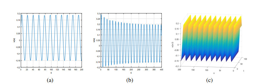
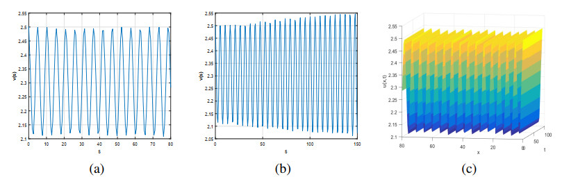
The existence, stability and bifurcation direction of periodic traveling waves for the Nicholson's blowflies model with delay and advection are investigated by applying the Hopf bifurcation theorem, center manifold theorem as well as normal form theory. Some numerical simulations are presented to illustrate our main results.
- Nicholson's blowflies model,
- delay,
- advection,
- periodic traveling waves,
- numerical simulations
Citation: Dong Li, Xiaxia Wu, Shuling Yan. Periodic traveling wave solutions of the Nicholson's blowflies model with delay and advection[J]. Electronic Research Archive, 2023, 31(5): 2568-2579. doi: 10.3934/era.2023130

Related Papers:

Abstract

The existence, stability and bifurcation direction of periodic traveling waves for the Nicholson's blowflies model with delay and advection are investigated by applying the Hopf bifurcation theorem, center manifold theorem as well as normal form theory. Some numerical simulations are presented to illustrate our main results.

References

[1]	[10.1111/j.1469-1809.1937.tb02153.x] R. Fisher, The wave of advance of advantageous genes, Ann. Hum. Genet., 7 (1937), 355–369. https://dx.doi.org/10.1111/j.1469-1809.1937.tb02153.x doi: 10.1111/j.1469-1809.1937.tb02153.x
[2]	I. Lundstr$\mathrm{\ddot{o}}$m, Mechanical wave propagation on nerve axons, J. Theor. Biol., 45 (1974), 487–499. https://doi.org/10.1016/0022-5193(74)90127-1 doi: 10.1016/0022-5193(74)90127-1
[3]	[10.1023/A: 1022616217603] J. Murray, Mathematical Biology. I. An Introduction, 3nd edition, New York: Springer-Verlag, 2002. http://dx.doi.org/10.1023/A: 1022616217603
[4]	W. Gurney, S. Blythe, R. Nisbet, Nicholson's blowflies revisited, Nature, 287 (1980), 17–21. https://doi.org/10.1038/287017a0 doi: 10.1038/287017a0
[5]	J. W. H. So, Y. Yang, Dirichlet problem for the diffusive Nicholson's blowflies equation, J. Differ. Equations, 150 (1998), 317–348. https://doi.org/10.1006/jdeq.1998.3489 doi: 10.1006/jdeq.1998.3489
[6]	J. W. H. So, X. Zou, Traveling waves for the diffusive Nicholson's blowflies equation, Appl. Math. Comput., 122 (2001), 385–392. https://doi.org/10.1016/S0096-3003(00)00055-2 doi: 10.1016/S0096-3003(00)00055-2
[7]	C. Lin, M. Mei, On travelling wavefronts of Nicholson's blowflies equation with diffusion, P. Roy. Soc. Edinb. A., 140 (2010), 135–152. https://doi.org/10.1017/S0308210508000784 doi: 10.1017/S0308210508000784
[8]	M. Mei, J. W. H. So, M. Li, S. Shen, Asymptotic stability of travelling waves for Nicholson's blowflies equation with diffusion, P. Roy. Soc. Edinb. A., 134 (2004), 579–594. https://doi.org/10.1017/S0308210500003358 doi: 10.1017/S0308210500003358
[9]	G. Yang, Hopf bifurcation of traveling wave of delayed Nicholson's blowflies equation, J. Biomath., 26 (2011), 81–86. https://doi.org/10.1016/j.amc.2013.06.051 doi: 10.1016/j.amc.2013.06.051
[10]	J. W. H. So, J. Wu, Y. Yang, Numerical steady state and Hopf bifurcation analysis on the diffusive Nicholson's blowflies equation, Appl. Math. Comput., 111 (2000), 53–69. https://doi.org/10.1016/S0096-3003(99)00047-8 doi: 10.1016/S0096-3003(99)00047-8
[11]	D. Duehring, W. Huang, Periodic traveling waves for diffusion equations with time delayed and non-local responding reaction, J. Dyn. Differ. Equations, 19 (2007), 457–477. https://doi.org/10.1007/s10884-006-9048-8 doi: 10.1007/s10884-006-9048-8
[12]	M. Mei, C. Lin, C. Lin, J. W. H. So, Traveling wavefronts for time-delayed reaction-diffusion equation: (I) local nonlinearity, J. Differ. Equations, 247 (2009), 495–510. https://doi.org/10.1016/j.jde.2008.12.026 doi: 10.1016/j.jde.2008.12.026
[13]	M. Mei, C. Ou, X. Zhao, Global stability of monostable traveling waves for nonlocal time-delayed reaction-diffusion equations, SIAM J. Math. Anal., 42 (2010), 2762–2790. https://doi.org/10.1137/090776342 doi: 10.1137/090776342
[14]	Z. Yang, G. Zhang, Global stability of traveling wavefronts for nonlocal reaction-diffusion equation with time delay, Acta Math. Sci., 38 (2018), 289–302. https://doi.org/10.3969/j.issn.0252-9602.2018.01.018 doi: 10.3969/j.issn.0252-9602.2018.01.018
[15]	J. Zhang, Y. Peng, Travelling waves of the diffusive Nicholson's blowflies equation with strong generic delay kernel and non-local effect, Nonlinear Anal.-Theor., 68 (2008), 1263–1270. https://doi.org/10.1016/j.na.2006.12.019 doi: 10.1016/j.na.2006.12.019
[16]	C. Huang, B. Liu, Traveling wave fronts for a diffusive Nicholsons Blowflies equation accompanying mature delay and feedback delay, Appl. Math. Lett., 134 (2022), 108321. https://doi.org/10.1016/j.aml.2022.108321 doi: 10.1016/j.aml.2022.108321
[17]	D. Liang, J. Wu, Travelling waves and numerical approximations in a reaction-diffusion equation with nonlocal delayed effect, J. Nonlinear Sci., 13 (2008), 289–310. https://doi.org/10.1007/s00332-003-0524-6 doi: 10.1007/s00332-003-0524-6
[18]	L. Liu, Y. Yang, S. Zhang, Stability of traveling fronts in a population model with nonlocal delay and advection, Malaya J. Mat., 3 (2015), 498–510.
[19]	Z. Wang, W. Li, S. Ruan, Existence and stability of traveling wave fronts in reaction advection diffusion equations with nonlocal delay, J. Differ. Equations, 238 (2007), 153–200. https://doi.org/10.1016/j.jde.2007.03.025 doi: 10.1016/j.jde.2007.03.025
[20]	S. Wu, W. Li, S. Liu, Exponential stability of traveling fronts in monostable reaction-advection-diffusion equations with non-local delay, Discrete Contin. Dyn. Syst. Ser. B., 17 (2012), 347–366. https://doi.org/10.3934/dcdsb.2012.17.347 doi: 10.3934/dcdsb.2012.17.347
[21]	H. Berestycki, The Influence of Advection on The Propagation of Fronts for Reaction-Diffusion Equations, Springer Netherlands, 2002. https://doi.org/10.1007/978-94-010-0307-02
[22]	D. Li, S. Guo, Periodic traveling waves in a reaction-diffusion model with chemotaxis and nonlocal delay effect, J. Math. Anal. Appl., 467 (2018), 1080–1099. https://doi.org/10.1016/j.jmaa.2018.07.050 doi: 10.1016/j.jmaa.2018.07.050
[23]	J. Hale, Theory of Functional Differential Equations, Springer-Verlag, New York, 1977. https://doi.org/10.1007/978-1-4612-9892-2

Reader Comments

Your name:*

Email:*
© 2023 the Author(s), licensee AIMS Press. This is an open access article distributed under the terms of the Creative Commons Attribution License (http://creativecommons.org/licenses/by/4.0)