Analysis of meningitis model: A case study of northern Nigeria

Isa Abdullahi Baba; Lawal Ibrahim Olamilekan; Abdullahi Yusuf; Dumitru Baleanu; Isa Abdullahi Baba; Lawal Ibrahim Olamilekan; Abdullahi Yusuf; Dumitru Baleanu

doi:10.3934/bioeng.2020016

AIMS Bioengineering

2020, Volume 7, Issue 4: 179-193. doi: 10.3934/bioeng.2020016

Previous Article Next Article

Research Article

Analysis of meningitis model: A case study of northern Nigeria

1.
Department of Mathematical Sciences, Bayero University, Kano, Nigeria
2.
Department of Computer Engineering, Biruni University, Istanbul Turkey
3.
Department of Mathematical Sciences, Federal University Dutse, Nigeria
4.
Department of Mathematics, Cankaya University, Ankara, 06530, Turkey
5.
Institute of Space Sciences, Bucharest, Romania
6.
Department of Medical Research, China Medical University Hospital, Taichung, Taiwan

Received: 09 May 2020 Accepted: 04 June 2020 Published: 24 June 2020

Abstract
Full Text(HTML)
Download PDF

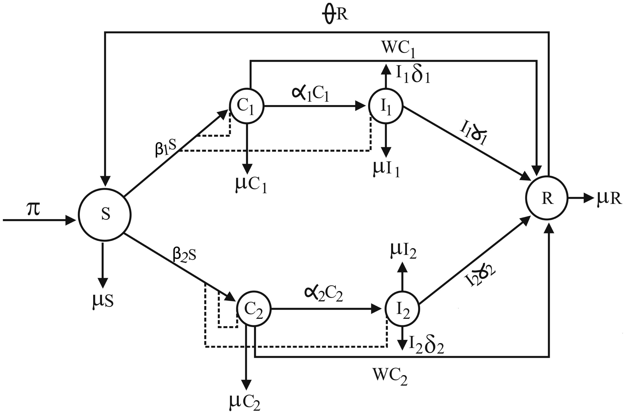
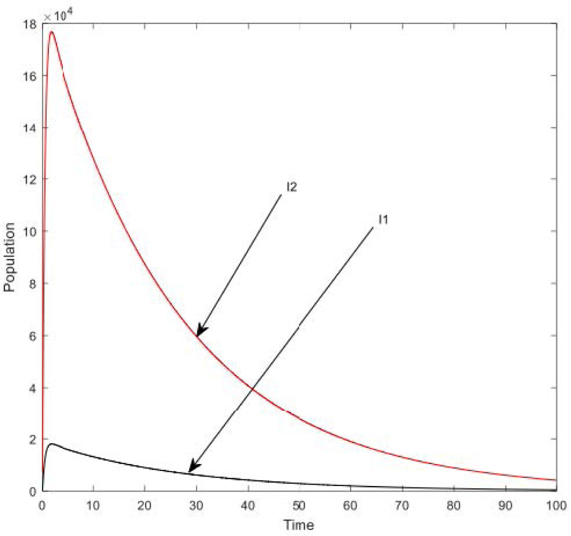
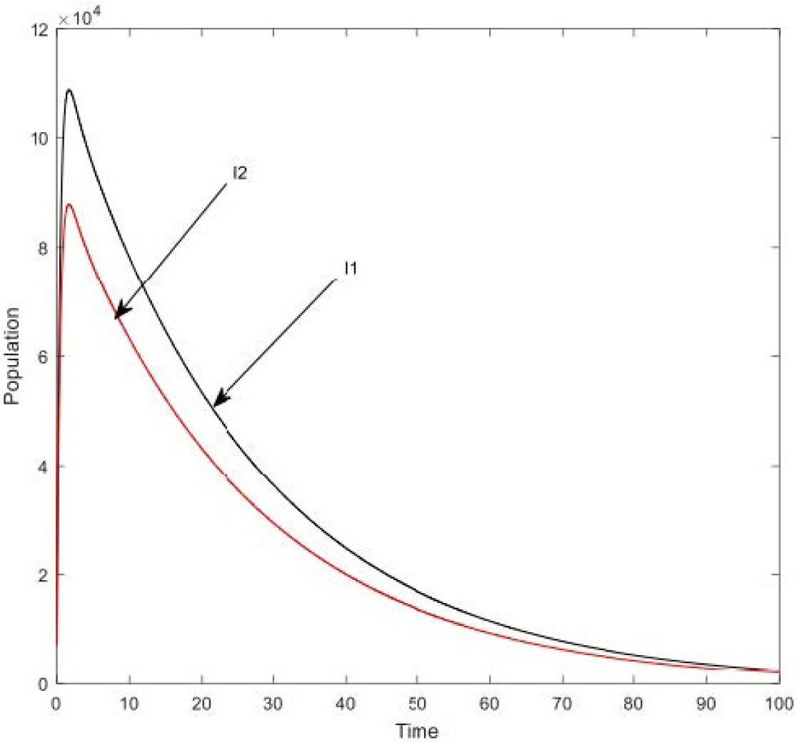
A new strain of meningitis emerges in northern Nigeria, which brought a lot of confusion. This is because vaccine and treatment for the old strain was adopted but to no avail. It was later discovered that it was a new strain that emerged. In this paper we consider the two strains of meningitis (I 1 and I 2). Our aim is to analyse the effect of one strain on the dynamics of the other strain mathematically. Equilibrium solutions were obtained and their global stability was analysed using Lyaponuv function. It was shown that the stability depends on magnitude of the basic reproduction ratio. The coexistence of the two strains was numerically shown.
- basic reproduction ratio,
- equilibrium solution,
- global stability,
- meningitis,
- two strain
Citation: Isa Abdullahi Baba, Lawal Ibrahim Olamilekan, Abdullahi Yusuf, Dumitru Baleanu. Analysis of meningitis model: A case study of northern Nigeria[J]. AIMS Bioengineering, 2020, 7(4): 179-193. doi: 10.3934/bioeng.2020016

Related Papers:

Abstract

A new strain of meningitis emerges in northern Nigeria, which brought a lot of confusion. This is because vaccine and treatment for the old strain was adopted but to no avail. It was later discovered that it was a new strain that emerged. In this paper we consider the two strains of meningitis (I 1 and I 2). Our aim is to analyse the effect of one strain on the dynamics of the other strain mathematically. Equilibrium solutions were obtained and their global stability was analysed using Lyaponuv function. It was shown that the stability depends on magnitude of the basic reproduction ratio. The coexistence of the two strains was numerically shown.

Acknowledgment

We would like to thank the reviewers for their useful suggestions.

Conflict of interest

Authors declare that they have no conflict of interest.

References

[1]	Howlett WP (2015) Neurology in Africa: Clinical Skills and Neurological Disorders UK: Cambridge University Press. doi: 10.1017/CBO9781316287064
[2]	Martínez MJF, Merino EG, Sánchez EG, et al. (2013) A mathematical model to study meningococcal meningitis. Procedia Comput Sci 18: 2492-2495. doi: 10.1016/j.procs.2013.05.426
[3]	(2017) CDC Centers for Disease control, Bacterial Meningitis. USA Available from: http//www.who.int/gho/epidemic_disease/meningitis/suspected_cases_death_text/en/.
[4]	Dushoff J, Plotkin JB, Levin SA, et al. (2004) Dynamical resonance can account for seasonal of influenza epidemic. Proc Natl Acd Sci USA 101: 16915-16916. doi: 10.1073/pnas.0407293101
[5]	Stone L, Olinky R, Huppert A (2007) Seasonal dynamic of recurrent epidemics. Nature 446: 533-536. doi: 10.1038/nature05638
[6]	Rvanchev LA (1968) Modeling experiment of a large epidemics by a means of computer. Trans USSR Acad Sci Ser Math Phy 180: 294-296.
[7]	Broutin H, Philippon S, De Magny GC, et al. (2007) Comparative study of meningitis dynamics across nine African countries: a global perceptive. Int J Health Geogr 6: 29. doi: 10.1186/1476-072X-6-29
[8]	Miller MA, Shahab CK (2005) Review of the cost effectiveness of immunization strategies for the control of epidemic meningococcal meningitis. Pharmacoeconomics 23: 333-343. doi: 10.2165/00019053-200523040-00004
[9]	Irving TJ, Blyuss KB, Colijn C, et al. (2012) Modeling meningococcal meningitis in the African meningitis belt. Epidemiol Infect 140: 897-905. doi: 10.1017/S0950268811001385
[10]	Kwambana-Adams BA, Amaza RC, Okoi C, et al. (2018) Meningococcus serogroup C clonal complex ST-10217 outbreak in Zamfara State, Northern Nigeria. Sci Rep 8: 14194. doi: 10.1038/s41598-018-32475-2
[11]	Chowell G, Miller MA, Viboud C (2008) Seasonal influenza in the United States, France and Australia: transmission and prospects for control. Epidemiol Infect 136: 852-864. doi: 10.1017/S0950268807009144
[12]	Bootsma MCJ, Ferguson NM (2007) The effect of public health measure on the 1918 influenza pandemic in US cities. Proc Natl Acad Sci USA 104: 7588-7593. doi: 10.1073/pnas.0611071104
[13]	Chowell G, Ammon CE, Hengartner NW, et al. (2006) Transmission dynamics of the great influenza pandemic of 1918 in Geneva, Switzerland: assessing the effect of hypothetical interventions. J Theor Biol 241: 193-204. doi: 10.1016/j.jtbi.2005.11.026
[14]	Mills CE, Robins JM, Lipstich M (2004) Transmissibility of 1918 pandemic influenza. Nature 432: 904-906. doi: 10.1038/nature03063
[15]	Chauchemez S, Valleron AJ, Boelle PY, et al. (2008) Estimating the impact of school closure on influenza transmission from Sentinel data. Nature 452: 750-754. doi: 10.1038/nature06732
[16]	Diekmann O, Heesterbeek JAP, Roberts MG (2010) The Construction of next-generation matrices for compartmental epidemic models. J R Soc Interface 7: 873-885. doi: 10.1098/rsif.2009.0386
[17]	Sene N (2020) SIR epidemic model with Mittag-Leffler fractional derivative. Chaos Soliton Fract 137: 109833. doi: 10.1016/j.chaos.2020.109833
[18]	Sene N (2019) Stability analysis of the generalized fractional differential equations with and without exogeneous inputs. J Nonlinear Sci Appl 12: 562-572. doi: 10.22436/jnsa.012.09.01
[19]	Sene N (2020) Global asymptotic stability of the fractional differential equations. J Nonlinear Sci Appl 13: 171-175.

Reader Comments

your name:*

Email:*
© 2020 the Author(s), licensee AIMS Press. This is an open access article distributed under the terms of the Creative Commons Attribution License (http://creativecommons.org/licenses/by/4.0)