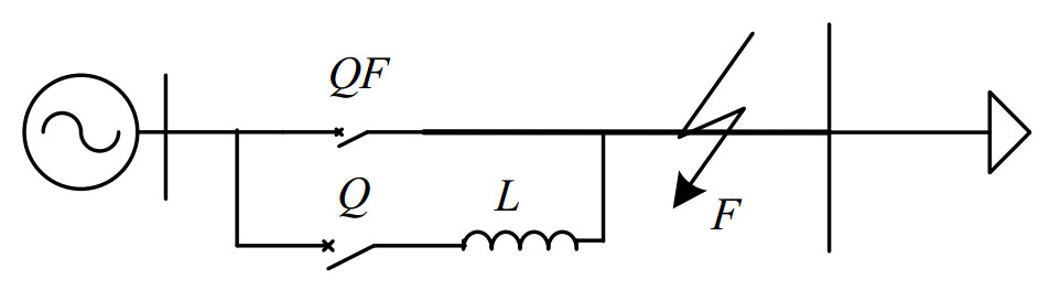
When a fault occurs on a distribution line, transient fault signals fade quickly, leaving only a short period of time for measurement and sampling. In addition, timing discrepancies between multiple measuring devices affect the accuracy of fault localization. This study proposes a method for fault detection in distribution lines based on an auxiliary inductance approach, where auxiliary inductors are introduced after the trip to provide steady-state fault data for localization. For asymmetrical short-circuit faults, the fault voltage is calculated from current and voltage measurements at both ends of the line, and the ratio of positive to negative sequence voltages is used to compensate for the phase angle and generate fault location functions. For symmetrical short-circuit faults, the voltage ratio between two faulted phases eliminates asynchronous angles, facilitating the derivation of fault location functions. Simulation results show that this method achieves high accuracy and is robust to differences in fault location, transition resistance, fault types, and synchronous angles.
Citation: Weiji Zhou, Jun Lin, Zekun Long, Feifei Liu, Mingfei He. Research on fault location method for distribution lines based on additional inductance strategy[J]. AIMS Energy, 2025, 13(2): 250-264. doi: 10.3934/energy.2025010
When a fault occurs on a distribution line, transient fault signals fade quickly, leaving only a short period of time for measurement and sampling. In addition, timing discrepancies between multiple measuring devices affect the accuracy of fault localization. This study proposes a method for fault detection in distribution lines based on an auxiliary inductance approach, where auxiliary inductors are introduced after the trip to provide steady-state fault data for localization. For asymmetrical short-circuit faults, the fault voltage is calculated from current and voltage measurements at both ends of the line, and the ratio of positive to negative sequence voltages is used to compensate for the phase angle and generate fault location functions. For symmetrical short-circuit faults, the voltage ratio between two faulted phases eliminates asynchronous angles, facilitating the derivation of fault location functions. Simulation results show that this method achieves high accuracy and is robust to differences in fault location, transition resistance, fault types, and synchronous angles.

| [1] |
Shu HC, Dai Y, An N, et al. (2023) Grounding electrode line fault location method based on simulation after test and deduction. Electr Power Syst Res 215: 108952. https://doi.org/10.1016/j.epsr.2022.108952 doi: 10.1016/j.epsr.2022.108952

|
| [2] |
Li Y, Wei X, Lin J, et al. (2023) A robust fault location method for active distribution network based on self-adaptive switching function. Int J Elec Power 148: 109007. https://doi.org/10.1016/j.ijepes.2023.109007 doi: 10.1016/j.ijepes.2023.109007
|
| [3] |
Liang Y, He A, Yuan J, et al. (2023) An accurate fault location method for distribution lines based on data fusion of outcomes from multiple algorithms. Int J Elec Power 153: 109290. https://doi.org/10.1016/j.ijepes.2023.109290 doi: 10.1016/j.ijepes.2023.109290
|
| [4] |
Wen J, Qu X, Liu J, et al. (2024) A novel fault location method for the active distribution network based on dynamic quantum genetic algorithm. Electr Eng 106: 4719–4735. https://doi.org/10.1007/s00202-024-02244-8 doi: 10.1007/s00202-024-02244-8
|
| [5] |
Mansourlakouraj M, Hosseinpour H, Livani H, et al. (2022) Waveform measurement unit-based fault location in distribution feeders via short-time matrix pencil method and graph neural network. IEEE Trans Ind Appl 59: 2661–2670. https://doi.org/10.1109/TIA.2022.3231586 doi: 10.1109/TIA.2022.3231586
|
| [6] |
Hu K, Cai Y, Cai Z, et al. (2022) Fault location method based on structure-preserving state estimation for distribution networks. Iet Gener Transm Dis 16: 3004–3015. https://doi.org/10.1049/gtd2.12492 doi: 10.1049/gtd2.12492
|
| [7] |
Bayati N, Mortensen LK, Savaghebi MSHR (2022) A localized transient-based fault location scheme for distribution systems. Sensonrs 22: 2723. https://doi.org/10.3390/s22072723 doi: 10.3390/s22072723
|
| [8] |
Wang C, Li P, Xu X, et al. (2022) A DC fault location method of multiterminal flexible DC distribution network. Math Probl Eng 2022: 8120857. https://doi.org/10.1155/2022/8120857 doi: 10.1155/2022/8120857
|
| [9] |
Rezaei D, Gholipour M, Parvaresh F (2022) A single-ended traveling-wave-based fault location for a hybrid transmission line using detected arrival times and TW' s polarity. Electr Pow Syst Res 210: 108058. https://doi.org/10.1016/j.epsr.2022.108058 doi: 10.1016/j.epsr.2022.108058
|
| [10] |
Kim SH (2022) Dimensionless impedance method for the transient response of pressurized pipeline system. Eng Appl Comp Fluid 16: 1641–1654. https://doi.org/10.1080/19942060.2022.2108500 doi: 10.1080/19942060.2022.2108500
|
| [11] |
Duarte N, Conti AD, Alipio R (2021) Assessment of ground-return impedance and admittance equations for the transient analysis of underground cables using a full-wave FDTD method. IEEE Trans Power Deliver 37: 3582–3589. https://doi.org/10.1109/TPWRD.2021.3131415 doi: 10.1109/TPWRD.2021.3131415
|
| [12] |
Won CY (2023) A virtual impedance-based flying start considering transient characteristics for permanent magnet synchronous machine drive systems. Energies 16: 1172. https://doi.org/10.3390/en16031172 doi: 10.3390/en16031172
|
| [13] |
Gomis-Bellmunt O, Song J, Cheah-Mane M, et al. (2022) Steady-state impedance mapping in grids with power electronics: What is grid strength in modern power systems? Int J Elec Power 136: 107635. https://doi.org/10.1016/j.ijepes.2021.107635 doi: 10.1016/j.ijepes.2021.107635
|
| [14] |
Monteiro FMDS, De Souza JV, Asada EN (2023) Analytical method to estimate the steady-state voltage impact of non-utility distributed energy resources. Electr Pow Syst Res 218: 109190. https://doi.org/10.1016/j.epsr.2023.109190 doi: 10.1016/j.epsr.2023.109190
|
| [15] |
Aquib M, Parth N, Doolla S, et al. (2023). An adaptive droop scheme for improving transient and steady-state power sharing among distributed generators in islanded microgrids. IEEE Trans Ind Appl 59: 5136–5148. https://doi.org/10.1109/TIA.2023.3272873 doi: 10.1109/TIA.2023.3272873
|
| [16] |
Wang S, Nie X, Li T, et al. (2024) Fast millimeter-wave three-dimensional holographic reconstruction based on target accurate distance. Opt Eng 63: 054104. https://doi.org/10.1117/1.OE.63.5.054104 doi: 10.1117/1.OE.63.5.054104
|
| [17] |
Deng LW, Lu JP, Shi JW, et al. (2020) A fault location method for hybrid lines based on two-terminal asynchronous data. Power Syst Technol 45: 1574–1580. https://doi.org/10.13335/j.1000-3673.pst.2020.0044a doi: 10.13335/j.1000-3673.pst.2020.0044a
|
| [18] |
Xie C, Li F, Fan Y, et al. (2019). Adaptive three-phase reclosing scheme of transmission lines without shunt reactors using additional capacitors. High Voltage Eng 45: 1811–1818. https://doi.org/10.13336/j.1003-6520.hve.20190604017 doi: 10.13336/j.1003-6520.hve.20190604017
|
| [19] |
Xiang L (2021) Key technology and application of primary and secondary fusion in distribution network. New Technol New Prod China 446: 66–68. https://doi.org/10.13612/j.cnki.cntp.2021.16.022 doi: 10.13612/j.cnki.cntp.2021.16.022
|
| [20] |
Liu J, Zhang Z, Rui J, et al. (2020) Adaptive reclosing of distribution lines based on primary and secondary device coordination. Power Syst Protec Control 48: 26–32. https://doi.org/10.19783/j.cnki.pspc.202084 doi: 10.19783/j.cnki.pspc.202084
|
| [21] |
Wang B, Cai L, Dong X, et al. (2017) A comprehensive analysis for asymmetrical short-circuit fault of electric power system with neutral-point unground. Prot Control Mod Pow 45: 149–153. https://doi.org/10.7667/PSPC160115 doi: 10.7667/PSPC160115
|
| [22] |
Hao W, Meng Z, Zhang Y, et al. (2023) Optimization model of the distribution network system by considering multi-types distributed power generation. J Jilin University 8: 1–11. https://doi.org/10.13229/j.cnki.jdxbgxb.20230119 doi: 10.13229/j.cnki.jdxbgxb.20230119
|


Figures(6) / Tables(4)

Weiji Zhou, Jun Lin, Zekun Long, Feifei Liu, Mingfei He. Research on fault location method for distribution lines based on additional inductance strategy[J]. AIMS Energy, 2025, 13(2): 250-264. doi: 10.3934/energy.2025010


 DownLoad: