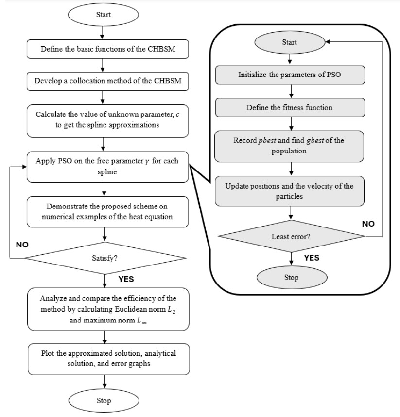
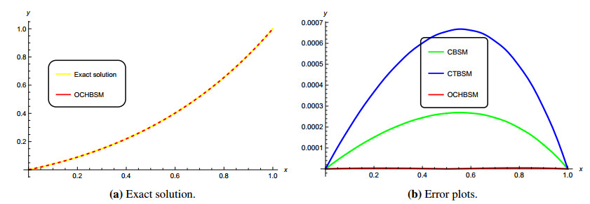
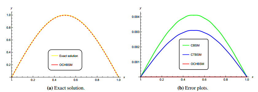
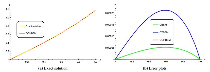
B-spline collocation methods were developed to provide simpler numerical solutions for differential problems. Over the years, various types of B-splines have been established, including the cubic B-spline collocation method (CBSM), cubic trigonometric B-spline collocation method (CTBSM), extended cubic B-spline collocation method (ECBSM), and cubic hybrid B-spline collocation method (CHBSM). Among these methods, CHBSM has been shown to produce the most accurate approximations due to the presence of a free parameter, $ \gamma $, which allows for greater flexibility in the basis functions. However, the accuracy of the CHBSM is highly dependent on the value of $ \gamma $, which must be optimized for improved results. While traditional brute-force optimization methods can achieve minimal errors, they often require significant computational time and effort. Therefore, this study has proposed using particle swarm optimization (PSO) to efficiently determine the optimal $ \gamma $ value for the CHBSM. The optimized CHBSM (OCHBSM) was tested on four examples of linear two-point boundary value problems (BVPs), including a linear BVP system. For comparison, the well-established CBSM and CTBSM were also applied to the same problems. The numerical results were analyzed and compared with analytical solutions revealing that the OCHBSM provided the most accurate approximations among the methods tested. Moreover, an average improvement percentage of 99.83% was achieved across all examples, indicating that our method outperforms the compared methods significantly.
Citation: Seherish Naz Khalid Ali Khan, Md Yushalify Misro. Hybrid B-spline collocation method with particle swarm optimization for solving linear differential problems[J]. AIMS Mathematics, 2025, 10(3): 5399-5420. doi: 10.3934/math.2025249
B-spline collocation methods were developed to provide simpler numerical solutions for differential problems. Over the years, various types of B-splines have been established, including the cubic B-spline collocation method (CBSM), cubic trigonometric B-spline collocation method (CTBSM), extended cubic B-spline collocation method (ECBSM), and cubic hybrid B-spline collocation method (CHBSM). Among these methods, CHBSM has been shown to produce the most accurate approximations due to the presence of a free parameter, $ \gamma $, which allows for greater flexibility in the basis functions. However, the accuracy of the CHBSM is highly dependent on the value of $ \gamma $, which must be optimized for improved results. While traditional brute-force optimization methods can achieve minimal errors, they often require significant computational time and effort. Therefore, this study has proposed using particle swarm optimization (PSO) to efficiently determine the optimal $ \gamma $ value for the CHBSM. The optimized CHBSM (OCHBSM) was tested on four examples of linear two-point boundary value problems (BVPs), including a linear BVP system. For comparison, the well-established CBSM and CTBSM were also applied to the same problems. The numerical results were analyzed and compared with analytical solutions revealing that the OCHBSM provided the most accurate approximations among the methods tested. Moreover, an average improvement percentage of 99.83% was achieved across all examples, indicating that our method outperforms the compared methods significantly.

| [1] | N. Asaithambi, Numerical Analysis: Theory and Practice, Saunders College Pub., 1995. |
| [2] |
S. Q. Wang, A variational approach to nonlinear two-point boundary value problems, Comput. Appl. Math., 58 (2009), 2452–2455. https://doi.org/10.1016/j.camwa.2009.03.050 doi: 10.1016/j.camwa.2009.03.050

|
| [3] |
Q. Fang, T. Tsuchiya, T. Yamamoto, Finite difference, finite element and finite volume methods applied to two-point boundary value problems, J. Comput. Appl. Math., 139 (2002), 9–19. https://doi.org/10.1016/s0377-0427(01)00392-2 doi: 10.1016/s0377-0427(01)00392-2
|
| [4] | S. Shafie, A. Majid, Approximation of cubic b-spline interpolation method, shooting and finite difference methods for linear problems on solving linear two-point boundary value problems, World Appl. Sci. J., 17 (2012), 1–9. |
| [5] |
H. Caglar, N. Caglar, K. Elfaituri, B-spline interpolation compared with finite difference, finite element and finite volume methods which applied to two-point boundary value problems, Appl. Math. Comput., 175 (2006), 72–79. https://doi.org/10.1016/j.amc.2005.07.019 doi: 10.1016/j.amc.2005.07.019
|
| [6] |
A. S. Heilat, R. S. Hailat, Extended cubic B-spline method for solving a system of non-linear second-order boundary value problems, J. Math. Comput. Sci., 21 (2020), 231–242. http://dx.doi.org/10.22436/jmcs.021.03.06 doi: 10.22436/jmcs.021.03.06
|
| [7] |
A. Khalid, A. Ghaffar, M. N. Naeem, K. S. Nisar, D. Baleanu, Solutions of bvps arising in hydrodynamic and magnetohydro-dynamic stability theory using polynomial and non-polynomial splines, Alex. Eng. J., 60 (2021), 941–953. https://doi.org/10.1016/j.aej.2020.10.022 doi: 10.1016/j.aej.2020.10.022
|
| [8] |
A. Tassaddiq, A. Khalid, M. N. Naeem, A. Ghaffar, F. Khan, S. A. A. Karim, et al., A new scheme using cubic B-spline to solve non-linear differential equations arising in visco-elastic flows and hydrodynamic stability problems, Mathematics, 7 (2019), 1078. https://doi.org/10.3390/math7111078 doi: 10.3390/math7111078
|
| [9] | N. N. Abd Hamid, A. A. Majid, A. I. M. Ismail, Extended cubic B-spline method for linear two-point boundary value problems, Sains Malaysiana, 40 (2011), 1285–1290. |
| [10] |
A. S. Heilat, A. I. M. Ismail, Hybrid cubic B-spline method for solving non-linear two-point boundary value problems, Int. J. Pure Appl. Math., 110 (2016), 369–381. https://doi.org/10.12732/ijpam.v110i2.11 doi: 10.12732/ijpam.v110i2.11
|
| [11] |
I. Wasim, M. Abbas, M. K. Iqbal, A new extended B-spline approximation technique for second order singular boundary value problems arising in physiology, J. Math. Comput. Sci., 19 (2019), 258–267. http://dx.doi.org/10.22436/jmcs.019.04.06 doi: 10.22436/jmcs.019.04.06
|
| [12] |
M. K. Iqbal, M. Abbas, I. Wasim, New cubic B-spline approximation for solving third order Emden–Flower type equations, Appl. Math. Comput., 331 (2018), 319–333. https://doi.org/10.1016/j.amc.2018.03.025 doi: 10.1016/j.amc.2018.03.025
|
| [13] |
M. Abbas, M. K. Iqbal, B. Zafar, S. B. M. Zin, New cubic B-spline approximations for solving non-linear third-order Korteweg-de Vries equation, Indian J. Sci. Technol., 12 (2019), 1–9. https://dx.doi.org/10.17485/ijst/2019/v12i6/141953 doi: 10.17485/ijst/2019/v12i6/141953
|
| [14] |
T. Nazir, M. Abbas. M. Iqbal, A new quintic B-spline approximation for numerical treatment of Boussinesq equation, J. Math. Comput. Sci., 20 (2020), 30–42. http://dx.doi.org/10.22436/jmcs.020.01.04 doi: 10.22436/jmcs.020.01.04
|
| [15] |
A. Ghaffar, M. Iqbal, M. Bari, S. Muhammad Hussain, R. Manzoor, K. Sooppy Nisar, et al., Construction and application of nine-tic B-spline tensor product ss, Mathematics, 7 (2019), 675. https://doi.org/10.3390/math7080675 doi: 10.3390/math7080675
|
| [16] | M. Iqbal, S. A. Abdul Karim, A. Shafie, M. Sarfraz, Convexity preservation of the ternary 6-point interpolating subdivision scheme, in Towards Intelligent Systems Modeling and Simulation: With Applications to Energy, Epidemiology and Risk Assessment, 383 (2021), 1–23. https://doi.org/10.1007/978-3-030-79606-8_1 |
| [17] |
M. Iqbal, N. Zainuddin, H. Daud, R. Kanan, R. Jusoh, A. Ullah, et al., Numerical solution of heat equation using modified cubic B-spline collocation method, J. Adv. Res. Numer. Heat Trans., 20 (2024), 23–35. https://doi.org/10.37934/arnht.20.1.2335 doi: 10.37934/arnht.20.1.2335
|
| [18] |
N. N. Abd Hamid, A. A. Majid, A. I. M. Ismail, Cubic trigonometric B-spline applied to linear two-point boundary value problems of order two, Int. J. Math. Comput. Sci., 4 (2010), 1377–1382. https://doi.org/10.5281/zenodo.1081989 doi: 10.5281/zenodo.1081989
|
| [19] |
A. S. Heilat, H. Zureigat, B. Batiha, New spline method for solving linear two-point boundary value problems, Eur. J. Pure Appl. Math., 14 (2021), 1283–1294. https://doi.org/10.29020/nybg.ejpam.v14i4.4124 doi: 10.29020/nybg.ejpam.v14i4.4124
|
| [20] |
S. Mat Zin, A. Abd Majid, A. I. M. Ismail, M. Abbas, Application of hybrid cubic B-spline collocation approach for solving a generalized nonlinear Klein-Gordon equation, Math. Probl. Eng., 2014 (2014), 108560. https://doi.org/10.1155/2014/108560 doi: 10.1155/2014/108560
|
| [21] | J. Kennedy, R. Eberhart, Particle swarm optimization, in Proceedings of ICNN'95-international conference on neural networks, 4 (1995), 1942–1948. http://dx.doi.org/10.1109/ICNN.1995.488968 |
| [22] |
R. Rani, G. Arora, H. Emadifar, M. Khademi, Numerical simulation of one-dimensional nonlinear Schrodinger equation using pso with exponential B-spline, Alex. Eng. J., 79 (2023), 644–651. https://doi.org/10.1016/j.aej.2023.08.050 doi: 10.1016/j.aej.2023.08.050
|
| [23] |
R. Rani, G. Arora, Particle swarm optimization numerical simulation with exponential modified cubic B-spline DQM, Int. J. Appl. Comput. Math., 10 (2024), 135. https://doi.org/10.1007/s40819-024-01697-6 doi: 10.1007/s40819-024-01697-6
|
| [24] |
J. Koupaei, M. Firouznia. S. Hosseini, Finding a good shape parameter of rbf to solve pdes based on the particle swarm optimization algorithm, Alex. Eng. J., 57 (2018), 3641–3652. https://doi.org/10.1016/j.aej.2017.11.024 doi: 10.1016/j.aej.2017.11.024
|
| [25] |
Z. Wu, X. Wang, Y. Fu, J. Shen, Q. Jiang, Y. Zhu, Fitting scattered data points with ball B-spline curves using particle swarm optimization, Comput. Graph., 72 (2018), 1–11. https://doi.org/10.1016/j.cag.2018.01.006 doi: 10.1016/j.cag.2018.01.006
|
| [26] |
S. Bibi, M. Y. Misro, M. Abbas, Shape optimization of GHT-Bézier developable surfaces using particle swarm optimization algorithm, Optim. Eng., 24 (2023), 1321–1341. https://doi.org/10.1007/s11081-022-09734-3 doi: 10.1007/s11081-022-09734-3
|
| [27] |
B. Latif, M. Y. Misro, S. A. Abdul Karim, I. Hashim, An improved symmetric numerical approach for systems of second-order two-point bvps, Symmetry, 15 (2023), 1166. https://doi.org/10.3390/sym15061166 doi: 10.3390/sym15061166
|
| [28] |
M. Iqbal, N. Zainuddin, H. Daud, R. Kanan, H. Soomro, R. Jusoh, et al., A modified basis of cubic B-spline with free parameter for linear second order boundary value problems: Application to engineering problems, J. King Saud Univ. Sci., 36 (2024), 103397. https://doi.org/10.1016/j.jksus.2024.103397 doi: 10.1016/j.jksus.2024.103397
|
| [29] | D. Salomon, Curves and surfaces for computer graphics, Springer Science & Business Media, 2007. |
| [30] |
M. Imran, R. Hashim, N. E. Abd Khalid, An overview of particle swarm optimization variants, Procedia Eng., 53 (2013), 491–496. https://doi.org/10.1016/j.proeng.2013.02.063 doi: 10.1016/j.proeng.2013.02.063
|
| [31] | A. Pradhan, S. K. Bisoy, Chapter 6 - inertia weight strategies for task allocation using metaheuristic algorithm, in BDCC, 2022,131–146. https://doi.org/10.1016/B978-0-323-85117-6.00004-2 |
| [32] |
W. Zhang, D. Ma, J. Wei, H. Liang, A parameter selection strategy for particle swarm optimization based on particle positions, Expert Syst. Appl., 41 (2014), 3576–3584. https://doi.org/10.1016/j.eswa.2013.10.061 doi: 10.1016/j.eswa.2013.10.061
|
| [33] |
M. E. Nordin, M. Y. Misro, Optimized bi-quadratic trigonometric Bézier curve using particle swarm optimization, ARASET, 33 (2023), 258–278. https://doi.org/10.37934/araset.33.3.258278 doi: 10.37934/araset.33.3.258278
|
| [34] |
J. Liu, X. Ren, H. Ma, A new pso algorithm with random c/d switchings, Appl. Math. Comput., 218 (2012), 9579–9593. https://doi.org/10.1016/j.amc.2012.02.059 doi: 10.1016/j.amc.2012.02.059
|
| [35] | S. N. K. A. Khan, B-spline collocation methods for linear two-point boundary Value problems, Master's thesis, School of Mathematical Sciences, Universiti Sains Malaysia, 2022. |
| [36] | R. L. Burden, Jd faires numerical analysis, Boston: Brooks-Cole. Pub, 672–674. |
| [37] | N. Hamid, A. Majid, A. Ismail, Cubic trigonometric B-spline applied to linear two-point boundary value problems of order two, Int. J. Math. Comput. Sci., 4 (2010), 1377–1382. |
| [38] |
N. Caglar, H. Caglar, B-spline method for solving linear system of second-order boundary value problems, Comput. Math. Appl., 57 (2009), 757–762. https://doi.org/10.1016/j.camwa.2008.09.033 doi: 10.1016/j.camwa.2008.09.033
|
| [39] |
A. S. Heilat, N. N. A. Hamid, A. I. M. Ismail, Extended cubic b-spline method for solving a linear system of second-order boundary value problems, Springerplus, 5 (2016), 1314. https://doi.org/10.1186/s40064-016-2936-4 doi: 10.1186/s40064-016-2936-4
|
Figures(5) / Tables(12)

Seherish Naz Khalid Ali Khan, Md Yushalify Misro. Hybrid B-spline collocation method with particle swarm optimization for solving linear differential problems[J]. AIMS Mathematics, 2025, 10(3): 5399-5420. doi: 10.3934/math.2025249


 DownLoad: