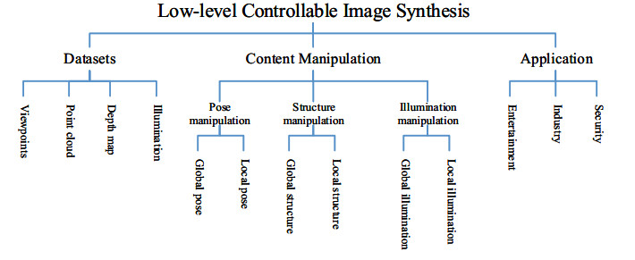
Deep learning, particularly generative models, has inspired controllable image synthesis methods and applications. These approaches aim to generate specific visual content using latent prompts. To explore low-level controllable image synthesis for precise rendering and editing tasks, we present a survey of recent works in this field using deep learning. We begin by discussing data sets and evaluation indicators for low-level controllable image synthesis. Then, we review the state-of-the-art research on geometrically controllable image synthesis, focusing on viewpoint/pose and structure/shape controllability. Additionally, we cover photometrically controllable image synthesis methods for 3D re-lighting studies. While our focus is on algorithms, we also provide a brief overview of related applications, products and resources for practitioners.
Citation: Shixiong Zhang, Jiao Li, Lu Yang. Survey on low-level controllable image synthesis with deep learning[J]. Electronic Research Archive, 2023, 31(12): 7385-7426. doi: 10.3934/era.2023374
Deep learning, particularly generative models, has inspired controllable image synthesis methods and applications. These approaches aim to generate specific visual content using latent prompts. To explore low-level controllable image synthesis for precise rendering and editing tasks, we present a survey of recent works in this field using deep learning. We begin by discussing data sets and evaluation indicators for low-level controllable image synthesis. Then, we review the state-of-the-art research on geometrically controllable image synthesis, focusing on viewpoint/pose and structure/shape controllability. Additionally, we cover photometrically controllable image synthesis methods for 3D re-lighting studies. While our focus is on algorithms, we also provide a brief overview of related applications, products and resources for practitioners.

| [1] | R. Rombach, A. Blattmann, D. Lorenz, P. Esser, B. Ommer, High-resolution image synthesis with latent diffusion models, in Proceedings of the IEEE/CVF Conference on Computer Vision and Pattern Recognition (CVPR), IEEE, (2022), 10684–10695. |
| [2] | Y. Cao, S. Li, Y. Liu, Z. Yan, Y. Dai, P. S. Yu, et al., A comprehensive survey of AI-generated content (aigc): A history of generative AI from GAN to ChatGPT, preprint, arXiv: 2303.04226. |
| [3] | R. Bommasani, D. A. Hudson, E. Adeli, R. Altman, S. Arora, S. V. Arx, et al., On the opportunities and risks of foundation models, preprint, arXiv: 2108.07258. |
| [4] | L. Zhang, A. Rao, M. Agrawala, Adding conditional control to text-to-image diffusion models, in Proceedings of the IEEE/CVF International Conference on Computer Vision (ICCV), IEEE, (2023), 3836–3847. |
| [5] | X. Wang, L. Xie, C. Dong, Y. Shan, Real-ESRGAN: Training real-world blind super-resolution with pure synthetic data, in Proceedings of the IEEE/CVF International Conference on Computer Vision Workshops (ICCVW), IEEE, (2021), 1905–1914. |
| [6] | H. Jonathan, J. Ajay, A. Pieter, Denoising diffusion probabilistic models, in Advances in Neural Information Processing Systems, Curran Associates, Inc., 33 (2020), 6840–6851. |
| [7] | I. J. Goodfellow, J. Pouget-Abadie, M. Mirza, B. Xu, D. Warde-Farley, S. Ozair, et al., Generative adversarial nets, in Advances in Neural Information Processing Systems, Curran Associates, Inc., 27 (2014), 1–9. |
| [8] | Y. LeCun, S. Chopra, R. Hadsell, M. Ranzato, F. Huang, A tutorial on energy-based learning, Predict. Struct. Data, 1 (2006), 1–59. |
| [9] |
J. Zhou, Z. Wu, Z. Jiang, K. Huang, K. Guo, S. Zhao, Background selection schema on deep learning-based classification of dermatological disease, Comput. Biol. Med., 149 (2022), 105966. https://doi.org/10.1016/j.compbiomed.2022.105966 doi: 10.1016/j.compbiomed.2022.105966

|
| [10] |
Q. Su, F. Wang, D. Chen, G. Chen, C. Li, L. Wei, Deep convolutional neural networks with ensemble learning and transfer learning for automated detection of gastrointestinal diseases, Comput. Biol. Med., 150 (2022), 106054. https://doi.org/10.1016/j.compbiomed.2022.106054 doi: 10.1016/j.compbiomed.2022.106054
|
| [11] |
G. Liu, Q. Ding, H. Luo, M. Sha, X. Li, M. Ju, Cx22: A new publicly available dataset for deep learning-based segmentation of cervical cytology images, Comput. Biol. Med., 150 (2022), 106194. https://doi.org/10.1016/j.compbiomed.2022.106194 doi: 10.1016/j.compbiomed.2022.106194
|
| [12] |
L. Xu, R. Magar, A. B. Farimani, Forecasting COVID-19 new cases using deep learning methods, Comput. Biol. Med., 144 (2022), 105342. https://doi.org/10.1016/j.compbiomed.2022.105342 doi: 10.1016/j.compbiomed.2022.105342
|
| [13] | D. P. Kingma, M. Welling, Auto-encoding variational bayes, preprint, arXiv: 1312.6114. |
| [14] | A. Radford, J. Wu, R. Child, D. Luan, D. Amodei, I. Sutskever, Language models are unsupervised multitask learners, OpenAI Blog, 1 (2019), 9. |
| [15] | H. Huang, P. S. Yu, C. Wang, An introduction to image synthesis with generative adversarial nets, preprint, arXiv: 1803.04469. |
| [16] | M. Mirza, S. Osindero, Conditional generative adversarial nets, preprint, arXiv: 1411.1784. |
| [17] | L. A. Gatys, A. S. Ecker, M. Bethge, Image style transfer using convolutional neural networks, in 2016 IEEE Conference on Computer Vision and Pattern Recognition (CVPR), IEEE, (2016), 2414–2423. https://doi.org/10.1109/CVPR.2016.265 |
| [18] | S. Agarwal, N. Snavely, I. Simon, S. M. Seitz, R. Szeliski, Building rome in a day, in 2009 IEEE 12th International Conference on Computer Vision, IEEE, (2009), 72–79. https://doi.org/10.1109/ICCV.2009.5459148 |
| [19] | L. Yang, T. Yendo, M. P. Tehrani, T. Fujii, M. Tanimoto, Probabilistic reliability based view synthesis for FTV, in 2010 IEEE International Conference on Image Processing, IEEE, (2010), 1785–1788. https://doi.org/10.1109/ICIP.2010.5650222 |
| [20] |
Y. Zheng, G. Zeng, H. Li, Q. Cai, J. Du, Colorful 3D reconstruction at high resolution using multi-view representation, J. Visual Commun. Image Represent., 85 (2022), 103486. https://doi.org/10.1016/j.jvcir.2022.103486 doi: 10.1016/j.jvcir.2022.103486
|
| [21] | J. Deng, W. Dong, R. Socher, L. Li, L. Kai, F. Li, ImageNet: A large-scale hierarchical image database, in 2009 IEEE Conference on Computer Vision and Pattern Recognition, IEEE, (2009), 248–255. https://doi.org/10.1109/CVPR.2009.5206848 |
| [22] | S. Christoph, B. Romain, V. Richard, G. Cade, W. Ross, C. Mehdi, et al., Laion-5b: An open large-scale dataset for training next generation image-text models, in Advances in Neural Information Processing Systems, Curran Associates, Inc., 35 (2022), 25278–25294. |
| [23] | S. M. Mohammad, S. Kiritchenko, Wikiart emotions: An annotated dataset of emotions evoked by art, in Proceedings of the 11th Edition of the Language Resources and Evaluation Conference (LREC-2018), (2018), 1–14. |
| [24] | M. Ben, P. P. Srinivasan, M. Tancik, J. T. Barron, R. Ramamoorthi, R. Ng, NeRF: Representing scenes as Neural Radiance Fields for view synthesis, in European Conference on Computer Vision, Springer, (2020), 405–421. https://doi.org/10.1007/978-3-030-58452-8_24 |
| [25] | S. Huang, Q. Li, J. Liao, L. Liu, L. Li, An overview of controllable image synthesis: Current challenges and future trends, SSRN, 2022. |
| [26] |
A. Tsirikoglou, G. Eilertsen, J. Unger, A survey of image synthesis methods for visual machine learning, Comput. Graphics Forum, 39 (2020), 426–451. https://doi.org/10.1111/cgf.14047 doi: 10.1111/cgf.14047
|
| [27] | H. Ren, G. Stella, B. S. Sami, Controllable GAN synthesis using non-rigid structure-from-motion, in Proceedings of the IEEE/CVF Conference on Computer Vision and Pattern Recognition, IEEE, (2023), 678–687. |
| [28] | J. Zhang, A. Siarohin, Y. Liu, H. Tang, N. Sebe, W. Wang, Training and tuning generative neural radiance fields for attribute-conditional 3D-aware face generation, preprint, arXiv: 2208.12550. |
| [29] | J. Ko, K. Cho, D. Choi, K. Ryoo, S. Kim, 3D GAN inversion with pose optimization, in Proceedings of the IEEE/CVF Winter Conference on Applications of Computer Vision (WACV), IEEE, (2023), 2967–2976. |
| [30] | S. Yang, W. Wang, B. Peng, J. Dong, Designing a 3D-aware StyleNeRF encoder for face editing, in ICASSP 2023–2023 IEEE International Conference on Acoustics, Speech and Signal Processing (ICASSP), IEEE, (2023), 1–5. https://doi.org/10.1109/ICASSP49357.2023.10094932 |
| [31] | J. Collins, S. Goel, K. Deng, A. Luthra, L. Xu, E. Gundogdu, et al., ABO: Dataset and benchmarks for real-world 3D object understanding, in Proceedings of the IEEE/CVF Conference on Computer Vision and Pattern Recognition, IEEE, (2022), 21126–21136. |
| [32] | B. Yang, Y. Zhang, Y. Xu, Y. Li, H. Zhou, H. Bao, et al., Learning object-compositional Neural Radiance Field for editable scene rendering, in 2021 IEEE/CVF International Conference on Computer Vision (ICCV), IEEE, (2021), 13759–13768. https://doi.org/10.1109/ICCV48922.2021.01352 |
| [33] | M. Niemeyer, A. Geiger, GIRAFFE: Representing scenes as compositional generative neural feature fields, in Proceedings of the IEEE/CVF Conference on Computer Vision and Pattern Recognition, IEEE, (2021), 11453–11464. |
| [34] | J. Zhu, C. Yang, Y. Shen, Z. Shi, B. Dai, D. Zhao, et al., LinkGAN: Linking GAN latents to pixels for controllable image synthesis, in Proceedings of the IEEE/CVF International Conference on Computer Vision (ICCV), IEEE, (2023), 7656–7666. |
| [35] | R. Gross, I. Matthews, J. Cohn, T. Kanade, S. Baker, Multi-PIE, in 2008 8th IEEE International Conference on Automatic Face and Gesture Recognition, IEEE, (2008), 1–8. https://doi.org/10.1109/AFGR.2008.4813399 |
| [36] | M. Boss, R. Braun, V. Jampani, J. T. Barron, C. Liu, H. P. A. Lensch, NeRD: Neural reflectance decomposition from image collections, in 2021 IEEE/CVF International Conference on Computer Vision (ICCV), IEEE, (2021), 12664–12674. https://doi.org/10.1109/ICCV48922.2021.01245 |
| [37] | X. Yan, Z. Yuan, Y. Du, Y. Liao, Y. Guo, Z. Li, et al., CLEVR3D: Compositional language and elementary visual reasoning for question answering in 3D real-world scenes, preprint, arXiv: 2112.11691. |
| [38] | A. Dai, A. X. Chang, M. Savva, M. Halber, T. Funkhouser, M. Nießner, ScanNet: Richly-annotated 3D reconstructions of indoor scenes, in Proceedings of the IEEE/CVF Conference on Computer Vision and Pattern Recognition, IEEE, (2017), 5828–5839. |
| [39] |
T. Zhou, T. Richard, F. John, F. Graham, S. Noah, Stereo magnification: Learning view synthesis using multiplane images, ACM Trans. Graphics, 37 (2018), 1–12. https://doi.org/10.1145/3197517.3201323 doi: 10.1145/3197517.3201323
|
| [40] | A. X. Chang, T. A. Funkhouser, L. J. Guibas, P. Hanrahan, Q. Huang, Z. Li, et al., ShapeNet: An information-rich 3D model repository, preprint, arXiv: 1512.03012. |
| [41] | A. Geiger, P. Lenz, R. Urtasun, Are we ready for autonomous driving? the KITTI vision benchmark suite, in 2012 IEEE Conference on Computer Vision and Pattern Recognition, IEEE, (2012), 3354–3361. https://doi.org/10.1109/CVPR.2012.6248074 |
| [42] | H. Caesar, V. Bankiti, A. H. Lang, S. Vora, V. E. Liong, Q. Xu, et al., NuScenes: A multimodal dataset for autonomous driving, in Proceedings of the IEEE/CVF Conference on Computer Vision and Pattern Recognition (CVPR), IEEE, (2020), 11621–11631. |
| [43] | S. K. Ramakrishnan, A. Gokaslan, E. Wijmans, O. Maksymets, A. Clegg, J. M. Turner, et al., Habitat-Matterport 3D dataset (HM3D): 1000 large-scale 3D environments for embodied AI, in Thirty-fifth Conference on Neural Information Processing Systems Datasets and Benchmarks Track (Round 2), (2021), 1–12. |
| [44] |
D. Scharstein, R. Szeliski, A taxonomy and evaluation of dense two-frame stereo correspondence algorithms, Int. J. Comput. Vision, 47 (2002), 7–42. https://doi.org/10.1023/A:1014573219977 doi: 10.1023/A:1014573219977
|
| [45] | D. Scharstein, R. Szeliski, High-accuracy stereo depth maps using structured light, in 2003 IEEE Computer Society Conference on Computer Vision and Pattern Recognition, IEEE, (2003), 1. https://doi.org/10.1109/CVPR.2003.1211354 |
| [46] | D. Scharstein, C. Pal, Learning conditional random fields for stereo, in 2007 IEEE Conference on Computer Vision and Pattern Recognition, IEEE, (2007), 1–8. https://doi.org/10.1109/CVPR.2007.383191 |
| [47] | H. Hirschmuller, D. Scharstein, Evaluation of cost functions for stereo matching, in 2007 IEEE Conference on Computer Vision and Pattern Recognition, IEEE, (2007), 1–8. https://doi.org/10.1109/CVPR.2007.383248 |
| [48] | D. Scharstein, H. Hirschmüller, Y. Kitajima, G. Krathwohl, N. Nesic, X. Wang, et al., High-resolution stereo datasets with subpixel-accurate ground truth, in 36th German Conference on Pattern Recognition, Springer, (2014), 31–42. https://doi.org/10.1007/978-3-319-11752-2_3 |
| [49] | N. Silberman, D. Hoiem, K. Pushmeet, R. Fergus, Indoor segmentation and support inference from rgbd images, in Computer Vision–ECCV 2012: 12th European Conference on Computer Vision, Springer, (2012), 746–760. https://doi.org/https://doi.org/10.1007/978-3-642-33715-4_54 |
| [50] |
K. Guo, P. Lincoln, P. Davidson, J. Busch, X. Yu, M. Whalen, et al., The Relightables: Volumetric performance capture of humans with realistic relighting, ACM Trans. Graphics, 38 (2019), 1–19. https://doi.org/10.1145/3355089.3356571 doi: 10.1145/3355089.3356571
|
| [51] | A. Horé, D. Ziou, Image quality metrics: PSNR vs. SSIM, in 2010 20th International Conference on Pattern Recognition, IEEE, (2010), 2366–2369. https://doi.org/10.1109/ICPR.2010.579 |
| [52] |
Z. Wang, A. C. Bovik, H. R. Sheikh, E. P. Simoncelli, Image quality assessment: From error visibility to structural similarity, IEEE Trans. Image Process., 13 (2004), 600–612. https://doi.org/10.1109/TIP.2003.819861 doi: 10.1109/TIP.2003.819861
|
| [53] | R. Zhang, P. Isola, A. A. Efros, E. Shechtman, O. Wang, The unreasonable effectiveness of deep features as a perceptual metric, in Proceedings of the IEEE conference on computer vision and pattern recognition, IEEE, (2018), 586–595. |
| [54] | T. Salimans, I. Goodfellow, W. Zaremba, V. Cheung, A. Radford, X. Chen, Improved techniques for training GANs, in Advances in Neural Information Processing Systems, Curran Associates, Inc., 29 (2016), 1–9. |
| [55] | M. Heusel, H. Ramsauer, T. Unterthiner, B. Nessler, S. Hochreiter, GANs trained by a two time-scale update rule converge to a local nash equilibrium, in Advances in Neural Information Processing Systems, Curran Associates Inc., 30 (2017), 1–12. |
| [56] | M. Bińkowski, D. J. Sutherland, M. Arbel, A. Gretton, Demystifying MMD GANs, in International Conference on Learning Representations, 2018. |
| [57] | Z. Shi, S. Peng, Y. Xu, Y. Liao, Y. Shen, Deep generative models on 3D representations: A survey, preprint, arXiv: 2210.15663. |
| [58] | R. Huang, S. Zhang, T. Li, R. He, Beyond face rotation: Global and local perception GAN for photorealistic and identity preserving frontal view synthesis, in Proceedings of the IEEE International Conference on Computer Vision (ICCV), IEEE, (2017), 2439–2448. |
| [59] | B. Zhao, X. Wu, Z. Cheng, H. Liu, Z. Jie, J. Feng, Multi-view image generation from a single-view, in Proceedings of the 26th ACM International Conference on Multimedia, ACM, (2018), 383–391. https://doi.org/10.1145/3240508.3240536 |
| [60] | K. Regmi, A. Borji, Cross-view image synthesis using conditional GANs, in 2018 IEEE/CVF Conference on Computer Vision and Pattern Recognition, IEEE, (2018), 3501–3510. https://doi.org/10.1109/CVPR.2018.00369 |
| [61] |
K. Regmi, A. Borji, Cross-view image synthesis using geometry-guided conditional GANs, Comput. Vision Image Understanding, 187 (2019), 102788. https://doi.org/10.1016/j.cviu.2019.07.008 doi: 10.1016/j.cviu.2019.07.008
|
| [62] | F. Mokhayeri, K. Kamali, E. Granger, Cross-domain face synthesis using a controllable GAN, in 2020 IEEE Winter Conference on Applications of Computer Vision (WACV), IEEE, (2020), 241–249. https://doi.org/10.1109/WACV45572.2020.9093275 |
| [63] | X. Zhu, Z. Yin, J. Shi, H. Li, D. Lin, Generative adversarial frontal view to bird view synthesis, in 2018 International Conference on 3D Vision (3DV), IEEE, (2018), 454–463. https://doi.org/10.1109/3DV.2018.00059 |
| [64] | H. Ding, S. Wu, H. Tang, F. Wu, G. Gao, X. Jing, Cross-view image synthesis with deformable convolution and attention mechanism, in Pattern Recognition and Computer Vision, Springer, (2020), 386–397. https://doi.org/10.1007/978-3-030-60633-6_32 |
| [65] | B. Ren, H. Tang, N. Sebe, Cascaded cross MLP-Mixer GANs for cross-view image translation, in British Machine Vision Conference, (2021), 1–14. |
| [66] | J. Zhu, T. Park, P. Isola, A. A. Efros, Unpaired image-to-image translation using cycle-consistent adversarial networks, in 2017 IEEE International Conference on Computer Vision (ICCV), IEEE, (2017), 2242–2251. https://doi.org/10.1109/ICCV.2017.244 |
| [67] | M. Yin, L. Sun, Q. Li, Novel view synthesis on unpaired data by conditional deformable variational auto-encoder, in Computer Vision–ECCV 2020, Springer, (2020), 87–103. https://doi.org/10.1007/978-3-030-58604-1_6 |
| [68] | X. Shen, J. Plested, Y. Yao, T. Gedeon, Pairwise-GAN: Pose-based view synthesis through pair-wise training, in Neural Information Processing, Springer, (2020), 507–515. https://doi.org/10.1007/978-3-030-63820-7_58 |
| [69] | E. R. Chan, M. Monteiro, P. Kellnhofer, J. Wu, G. Wetzstein, pi-GAN: Periodic implicit generative adversarial networks for 3D-aware image synthesis, in 2021 IEEE/CVF Conference on Computer Vision and Pattern Recognition (CVPR), IEEE, (2021), 5795–5805. https://doi.org/10.1109/CVPR46437.2021.00574 |
| [70] | S. Cai, A. Obukhov, D. Dai, L. V. Gool, Pix2NeRF: Unsupervised conditional $\pi$-GAN for single image to Neural Radiance Fields translation, in 2022 IEEE/CVF Conference on Computer Vision and Pattern Recognition (CVPR), IEEE, (2022), 3971–3980. https://doi.org/10.1109/CVPR52688.2022.00395 |
| [71] |
T. Leimkhler, G. Drettakis, FreeStyleGAN, ACM Trans. Graphics, 40 (2021), 1–15. https://doi.org/10.1145/3478513.3480538 doi: 10.1145/3478513.3480538
|
| [72] | S. C. Medin, B. Egger, A. Cherian, Y. Wang, J. B. Tenenbaum, X. Liu, et al., MOST-GAN: 3D morphable StyleGAN for disentangled face image manipulation, in Proceedings of the AAAI Conference on Artificial Intelligence, AAAI Press, 36 (2022), 1962–1971. https://doi.org/10.1609/aaai.v36i2.20091 |
| [73] | R. Or-El, X. Luo, M. Shan, E. Shechtman, J. J. Park, I. Kemelmacher-Shlizerman, StyleSDF: High-resolution 3D-consistent image and geometry generation, in Proceedings of the IEEE/CVF Conference on Computer Vision and Pattern Recognition (CVPR), IEEE, (2022), 13503–13513. |
| [74] |
X. Zheng, Y. Liu, P. Wang, X. Tong, SDF-StyleGAN: Implicit SDF-based StyleGAN for 3D shape generation, Comput. Graphics Forum, 41 (2022), 52–63. https://doi.org/10.1111/cgf.14602 doi: 10.1111/cgf.14602
|
| [75] | Y. Deng, J. Yang, J. Xiang, X. Tong, GRAM: Generative radiance manifolds for 3D-aware image generation, in 2022 IEEE/CVF Conference on Computer Vision and Pattern Recognition, IEEE, (2022), 10663–10673. https://doi.org/10.1109/CVPR52688.2022.01041 |
| [76] | J. Xiang, J. Yang, Y. Deng, X. Tong, GRAM-HD: 3D-consistent image generation at high resolution with generative radiance manifolds, in Proceedings of the IEEE/CVF International Conference on Computer Vision (ICCV), IEEE, (2023), 2195–2205. |
| [77] | E. R. Chan, C. Z. Lin, M. A. Chan, K. Nagano, B. Pan, S. D. Mello, et al., Efficient geometry-aware 3D generative adversarial networks, in Proceedings of the IEEE/CVF Conference on Computer Vision and Pattern Recognition (CVPR), IEEE, (2022), 16123–16133. |
| [78] | X. Zhao, F. Ma, D. Güera, Z. Ren, A. G. Schwing, A. Colburn, Generative multiplane images: Making a 2D GAN 3D-aware, in Computer Vision–ECCV 2022, Springer, (2022), 18–35. https://doi.org/10.1007/978-3-031-20065-6_2 |
| [79] | H. A. Alhaija, A. Dirik, A. Knrig, S. Fidler, M. Shugrina, XDGAN: Multi-modal 3D shape generation in 2D space, in British Machine Vision Conference, (2022), 1–14. |
| [80] | K. Zhang, G. Riegler, N. Snavely, V. Koltun, NeRF++: Analyzing and improving Neural Radiance Fields, preprint, arXiv: 2010.07492. |
| [81] | D. Rebain, W. Jiang, S. Yazdani, K. Li, K. M. Yi, A. Tagliasacchi, DeRF: Decomposed radiance fields, in 2021 IEEE/CVF Conference on Computer Vision and Pattern Recognition (CVPR), IEEE, (2021), 14148–14156. https://doi.org/10.1109/CVPR46437.2021.01393 |
| [82] | K. Park, U. Sinha, J. T. Barron, S. Bouaziz, D. B. Goldman, S. M. Seitz, et al., Nerfies: Deformable Neural Radiance Fields, in 2021 IEEE/CVF International Conference on Computer Vision (ICCV), IEEE, (2021), 5845–5854. https://doi.org/10.1109/ICCV48922.2021.00581 |
| [83] | J. Li, Z. Feng, Q. She, H. Ding, C. Wang, G. H. Lee, MINE: Towards continuous depth MPI with NeRF for novel view synthesis, in 2021 IEEE/CVF International Conference on Computer Vision (ICCV), IEEE, (2021), 12558–12568. https://doi.org/10.1109/ICCV48922.2021.01235 |
| [84] |
K. Park, U. Sinha, P. Hedman, J. T. Barron, S. Bouaziz, D. B. Goldman, et al., HyperNeRF: A higher-dimensional representation for topologically varying Neural Radiance Fields, ACM Trans. Graphics, 40 (2021), 1–12. https://doi.org/10.1145/3478513.3480487 doi: 10.1145/3478513.3480487
|
| [85] | T. Chen, P. Wang, Z. Fan, Z. Wang, Aug-NeRF: Training stronger Neural Radiance Fields with triple-level physically-grounded augmentations, in 2022 IEEE/CVF Conference on Computer Vision and Pattern Recognition (CVPR), IEEE, (2022), 15170–15181. https://doi.org/10.1109/CVPR52688.2022.01476 |
| [86] | T. Kaneko, AR-NeRF: Unsupervised learning of depth and defocus effects from natural images with aperture rendering Neural Radiance Fields, in Proceedings of the IEEE/CVF Conference on Computer Vision and Pattern Recognition (CVPR), IEEE, (2022), 18387–18397. |
| [87] | X. Li, C. Hong, Y. Wang, Z. Cao, K. Xian, G. Lin, SymmNeRF: Learning to explore symmetry prior for single-view view synthesis, in Proceedings of the Asian Conference on Computer Vision (ACCV), (2022), 1726–1742. |
| [88] | K. Zhou, W. Li, Y. Wang, T. Hu, N. Jiang, X. Han, et al., NeRFLix: High-quality neural view synthesis by learning a degradation-driven inter-viewpoint mixer, in Proceedings of the IEEE/CVF Conference on Computer Vision and Pattern Recognition (CVPR), IEEE, (2023), 12363–12374. |
| [89] | Z. Wang, S. Wu, W. Xie, M. Chen, V. A. Prisacariu, NeRF–: Neural Radiance Fields without known camera parameters, preprint, arXiv: 2102.07064. |
| [90] |
B. Mildenhall, P. P. Srinivasan, R. Ortiz-Cayon, N. K. Kalantari, R. Ramamoorthi, R. Ng, et al., Local light field fusion: Practical view synthesis with prescriptive sampling guidelines, ACM Trans. Graphics, 38 (2019), 1–14. https://doi.org/10.1145/3306346.3322980 doi: 10.1145/3306346.3322980
|
| [91] | Q. Meng, A. Chen, H. Luo, M. Wu, H. Su, L. Xu, et al., GNeRF: GAN-based Neural Radiance Field without posed camera, in Proceedings of the IEEE/CVF International Conference on Computer Vision (ICCV), IEEE, (2021), 6351–6361. |
| [92] | R. Jensen, A. Dahl, G. Vogiatzis, E. Tola, H. Aanæs, Large scale multi-view stereopsis evaluation, in Proceedings of the 2014 IEEE Conference on Computer Vision and Pattern Recognition, IEEE, (2014), 406–413. https://doi.org/10.1109/CVPR.2014.59 |
| [93] | Y. Jeong, S. Ahn, C. Choy, A. Anandkumar, M. Cho, J. Park, Self-calibrating Neural Radiance Fields, in 2021 IEEE/CVF International Conference on Computer Vision (ICCV), IEEE, (2021), 5826–5834. https://doi.org/10.1109/ICCV48922.2021.00579 |
| [94] |
A. Knapitsch, J. Park, Q. Zhou, V. Koltun, Tanks and temples: Benchmarking large-scale scene reconstruction, ACM Trans. Graphics, 36 (2017), 1–13. https://doi.org/10.1145/3072959.3073599 doi: 10.1145/3072959.3073599
|
| [95] | W. Bian, Z. Wang, K. Li, J. Bian, V. A. Prisacariu, NoPe-NeRF: Optimising Neural Radiance Field with no pose prior, in Proceedings of the IEEE/CVF Conference on Computer Vision and Pattern Recognition (CVPR), IEEE, (2023), 4160–4169. |
| [96] | P. Truong, M. Rakotosaona, F. Manhardt, F. Tombari, SPARF: Neural Radiance Fields from sparse and noisy poses, in Proceedings of the IEEE/CVF Conference on Computer Vision and Pattern Recognition (CVPR), IEEE, (2023), 4190–4200. |
| [97] | J. Straub, T. Whelan, L. Ma, Y. Chen, E. Wijmans, S. Green, et al., The replica dataset: A digital replica of indoor spaces, preprint, arXiv: 1906.05797. |
| [98] | J. Y. Zhang, G. Yang, S. Tulsiani, D. Ramanan, NeRS: Neural reflectance surfaces for sparse-view 3D reconstruction in the wild, in Conference on Neural Information Processing Systems, Curran Associates, Inc., 34 (2021), 29835–29847. |
| [99] | S. Seo, D. Han, Y. Chang, N. Kwak, MixNeRF: Modeling a ray with mixture density for novel view synthesis from sparse inputs, in Proceedings of the IEEE/CVF Conference on Computer Vision and Pattern Recognition (CVPR), IEEE, (2023), 20659–20668. |
| [100] | A. Cao, R. D. Charette, SceneRF: Self-supervised monocular 3D scene reconstruction with radiance fields, in Proceedings of the IEEE/CVF International Conference on Computer Vision (ICCV), IEEE, (2023), 9387–9398. |
| [101] | J. Behley, M. Garbade, A. Milioto, J. Quenzel, S. Behnke, C. Stachniss, et al., SemanticKITTI: A dataset for semantic scene understanding of lidar sequences, in 2019 IEEE/CVF International Conference on Computer Vision (ICCV), IEEE, (2019), 9296–9306. https://doi.org/10.1109/ICCV.2019.00939 |
| [102] | J. Chen, W. Yi, L. Ma, X. Jia, H. Lu, GM-NeRF: Learning generalizable model-based Neural Radiance Fields from multi-view images, in Proceedings of the IEEE/CVF Conference on Computer Vision and Pattern Recognition (CVPR), IEEE, (2023), 20648–20658. |
| [103] | T. Yu, Z. Zheng, K. Guo, P. Liu, Q. Dai, Y. Liu, Function4D: Real-time human volumetric capture from very sparse consumer rgbd sensors, in 2021 IEEE/CVF Conference on Computer Vision and Pattern Recognition (CVPR), IEEE, (2021), 5742–5752. https://doi.org/10.1109/CVPR46437.2021.00569 |
| [104] | B. Bhatnagar, G. Tiwari, C. Theobalt, G. Pons-Moll, Multi-Garment net: Learning to dress 3D people from images, in 2019 IEEE/CVF International Conference on Computer Vision (ICCV), IEEE, (2019), 5419–5429. https://doi.org/10.1109/ICCV.2019.00552 |
| [105] | W. Cheng, S. Xu, J. Piao, C. Qian, W. Wu, K. Lin, et al., Generalizable neural performer: Learning robust radiance fields for human novel view synthesis, preprint, arXiv: 2204.11798. |
| [106] | S. Peng, Y. Zhang, Y. Xu, Q. Wang, Q. Shuai, H. Bao, et al., Neural Body: Implicit neural representations with structured latent codes for novel view synthesis of dynamic humans, in 2021 IEEE/CVF Conference on Computer Vision and Pattern Recognition (CVPR), IEEE, (2021), 9050–9059. https://doi.org/10.1109/CVPR46437.2021.00894 |
| [107] | B. Mildenhall, P. Hedman, R. Martin-Brualla, P. P. Srinivasan, J. T. Barron, NeRF in the dark: High dynamic range view synthesis from noisy raw images, in Proceedings of the IEEE/CVF Conference on Computer Vision and Pattern Recognition (CVPR), IEEE, (2022), 16190–16199. |
| [108] | L. Ma, X. Li, J. Liao, Q. Zhang, X. Wang, J. Wang, et al., Deblur-NeRF: Neural Radiance Fields from blurry images, in Proceedings of the IEEE/CVF Conference on Computer Vision and Pattern Recognition (CVPR), IEEE, (2022), 12861–12870. |
| [109] | X. Huang, Q. Zhang, Y. Feng, H. Li, X. Wang, Q. Wang, Hdr-NeRF: High dynamic range Neural Radiance Fields, in Proceedings of the IEEE/CVF Conference on Computer Vision and Pattern Recognition, IEEE, (2022), 18398–18408. |
| [110] | P. Naama, T. Tali, K. Simon, NAN: Noise-aware NeRFs for burst-denoising, in Proceedings of the IEEE/CVF Conference on Computer Vision and Pattern Recognition (CVPR), IEEE, (2022), 12672–12681. |
| [111] | J. T. Barron, B. Mildenhall, D. Verbin, P. P. Srinivasan, P. Hedman, Mip-NeRF 360: Unbounded anti-aliased Neural Radiance Fields, in Proceedings of the IEEE/CVF Conference on Computer Vision and Pattern Recognition (CVPR), IEEE, (2022), 5470–5479. |
| [112] | Y. Xiangli, L. Xu, X. Pan, N. Zhao, A. Rao, C. Theobalt, et al., BungeeNeRF: Progressive Neural Radiance Field for extreme multi-scale scene rendering, in Computer Vision–ECCV 2022, Springer, (2022), 106–122. https://doi.org/10.1007/978-3-031-19824-3_7 |
| [113] | Google, Google earth studio, 2018. Available from: https://www.google.com/earth/studio/. |
| [114] | M. Tancik, V. Casser, X. Yan, S. Pradhan, B. P. Mildenhall, P. Srinivasan, et al., Block-NeRF: Scalable large scene neural view synthesis, in 2022 IEEE/CVF Conference on Computer Vision and Pattern Recognition (CVPR), IEEE, (2022), 8238–8248. https://doi.org/10.1109/CVPR52688.2022.00807 |
| [115] | L. Xu, Y. Xiangli, S. Peng, X. Pan, N. Zhao, C. Theobalt, et al., Grid-guided Neural Radiance Fields for large urban scenes, in Proceedings of the IEEE/CVF Conference on Computer Vision and Pattern Recognition (CVPR), IEEE, (2023), 8296–8306. |
| [116] | T. Haithem, R. Deva, S. Mahadev, Mega-NERF: Scalable construction of large-scale NeRFs for virtual fly-throughs, in Proceedings of the IEEE/CVF Conference on Computer Vision and Pattern Recognition (CVPR), IEEE, (2022), 12922–12931. |
| [117] | C. Choi, S. M. Kim, Y. M. Kim, Balanced spherical grid for egocentric view synthesis, in Proceedings of the IEEE/CVF Conference on Computer Vision and Pattern Recognition (CVPR), IEEE, (2022), 16590–16599. |
| [118] | A. Yu, R. Li, M. Tancik, H. Li, R. Ng, A. Kanazawa, PlenOctrees for real-time rendering of Neural Radiance Fields, in 2021 IEEE/CVF International Conference on Computer Vision (ICCV), IEEE, (2021), 5732–5741. https://doi.org/10.1109/ICCV48922.2021.00570 |
| [119] | C. Sun, M. Sun, H. Chen, Direct voxel grid optimization: Super-fast convergence for radiance fields reconstruction, in 2022 IEEE/CVF Conference on Computer Vision and Pattern Recognition (CVPR), IEEE, (2022), 5449–5459. https://doi.org/10.1109/CVPR52688.2022.00538 |
| [120] | L. Liu, J. Gu, K. Z. Lin, T. Chua, C. Theobalt, Neural sparse voxel fields, in Advances in Neural Information Processing Systems, Curran Associates, Inc., 33 (2020), 15651–15663. |
| [121] | Y. Yao, Z. Luo, S. Li, J. Zhang, Y. Ren, L. Zhou, et al., BlendedMVS: A large-scale dataset for generalized multi-view stereo networks, in Proceedings of the IEEE/CVF Conference on Computer Vision and Pattern Recognition (CVPR), IEEE, (2020), 1790–1799. |
| [122] | V. Sitzmann, J. Thies, F. Heide, M. Nießner, G. Wetzstein, M. Zollhöfer, DeepVoxels: Learning persistent 3D feature embeddings, in Proceedings of the IEEE/CVF Conference on Computer Vision and Pattern Recognition (CVPR), IEEE, (2019), 2437–2446. |
| [123] | H. Wang, J. Ren, Z. Huang, K. Olszewski, M. Chai, Y. Fu, et al., R2L: Distilling Neural Radiance Field to neural light field for efficient novel view synthesis, in Computer Vision–ECCV 2022, Springer, (2022), 612–629. https://doi.org/10.1007/978-3-031-19821-2_35 |
| [124] |
T. Neff, P. Stadlbauer, M. Parger, A. Kurz, J. H. Mueller, C. R. A. Chaitanya, et al., DONeRF: Towards real-time rendering of compact Neural Radiance Fields using depth oracle networks, Comput. Graphics Forum, 40 (2021), 45–59. https://doi.org/10.1111/cgf.14340 doi: 10.1111/cgf.14340
|
| [125] | K. Wadhwani, T. Kojima, SqueezeNeRF: Further factorized FastNeRF for memory-efficient inference, in 2022 IEEE/CVF Conference on Computer Vision and Pattern Recognition Workshops (CVPRW), IEEE, (2022), 2716–2724. https://doi.org/10.1109/CVPRW56347.2022.00307 |
| [126] | Z. Chen, T. Funkhouser, P. Hedman, A. Tagliasacchi, MobileNeRF: Exploiting the polygon rasterization pipeline for efficient neural field rendering on mobile architectures, in Proceedings of the IEEE/CVF Conference on Computer Vision and Pattern Recognition, IEEE, (2023), 16569–16578. |
| [127] | Y. Chen, X. Chen, X. Wang, Q. Zhang, Y. Guo, Y. Shan, et al., Local-to-global registration for bundle-adjusting Neural Radiance Fields, in Proceedings of the IEEE/CVF Conference on Computer Vision and Pattern Recognition, IEEE, (2023), 8264–8273. |
| [128] | C. Sbrolli, P. Cudrano, M. Frosi, M. Matteucci, IC3D: Image-conditioned 3D diffusion for shape generation, preprint, arXiv: 2211.10865. |
| [129] | J. Gu, Q. Gao, S. Zhai, B. Chen, L. Liu, J. Susskind, Learning controllable 3D diffusion models from single-view images, preprint, arXiv: 2304.06700. |
| [130] | T. Anciukevičius, Z. Xu, M. Fisher, P. Henderson, H. Bilen, N. J. Mitra, et al., RenderDiffusion: Image diffusion for 3D reconstruction, inpainting and generation, in Proceedings of the IEEE/CVF Conference on Computer Vision and Pattern Recognition (CVPR), IEEE, (2023), 12608–12618. |
| [131] | J. Xiang, J. Yang, B. Huang, X. Tong, 3D-aware image generation using 2D diffusion models, in Proceedings of the IEEE/CVF International Conference on Computer Vision (ICCV), IEEE, (2023), 2383–2393. |
| [132] | R. Liu, R. Wu, B. V. Hoorick, P. Tokmakov, S. Zakharov, C. Vondrick, Zero-1-to-3: Zero-shot one image to 3D object, preprint, arXiv: 2303.11328. |
| [133] | E. R. Chan, K. Nagano, M. A. Chan, A. W. Bergman, J. J. Park, A. Levy, et al., Generative novel view synthesis with 3D-aware diffusion models, in Proceedings of the IEEE/CVF International Conference on Computer Vision (ICCV), IEEE, (2023), 4217–4229. |
| [134] | A. Dosovitskiy, L. Beyer, A. Kolesnikov, D. Weissenborn, X. Zhai, T. Unterthiner, et al., An image is worth 16 x 16 words: Transformers for image recognition at scale, in International Conference on Learning Representations, 2021. |
| [135] | A. Vaswani, N. Shazeer, N. Parmar, J. Uszkoreit, L. Jones, A. N. Gomez, et al., Attention is all you need, in Proceedings of the 31st International Conference on Neural Information Processing Systems, Curran Associates Inc., (2017), 6000–6010. |
| [136] | P. Nguyen-Ha, L. Huynh, E. Rahtu, J. Heikkila, Sequential view synthesis with transformer, in Proceedings of the Asian Conference on Computer Vision (ACCV), 2020. |
| [137] |
J. Yang, Y. Li, L. Yang, Shape transformer nets: Generating viewpoint-invariant 3D shapes from a single image, J. Visual Commun. Image Represent., 81 (2021), 103345. https://doi.org/10.1016/j.jvcir.2021.103345 doi: 10.1016/j.jvcir.2021.103345
|
| [138] | J. Kulhánek, E. Derner, T. Sattler, R. Babuška, ViewFormer: NeRF-free neural rendering from few images using transformers, in Computer Vision–ECCV 2022, Springer, (2022), 198–216. https://doi.org/10.1007/978-3-031-19784-0_12 |
| [139] | P. Zhou, L. Xie, B. Ni, Q. Tian, CIPS-3D: A 3D-aware generator of GANs based on conditionally-independent pixel synthesis, preprint, arXiv: 2110.09788. |
| [140] | X. Xu, X. Pan, D. Lin, B. Dai, Generative occupancy fields for 3D surface-aware image synthesis, in Advances in Neural Information Processing Systems, Curran Associates, Inc., 34 (2021), 20683–20695. |
| [141] | Y. Lan, X. Meng, S. Yang, C. C. Loy, B. Dai, Self-supervised geometry-aware encoder for style-based 3D GAN inversion, in Proceedings of the IEEE/CVF Conference on Computer Vision and Pattern Recognition (CVPR), IEEE, (2023), 20940–20949. |
| [142] | S. Li, J. van de Weijer, Y. Wang, F. S. Khan, M. Liu, J. Yang, 3D-aware multi-class image-to-image translation with NeRFs, in Proceedings of the IEEE/CVF Conference on Computer Vision and Pattern Recognition (CVPR), IEEE, (2023), 12652–12662. |
| [143] | M. Shahbazi, E. Ntavelis, A. Tonioni, E. Collins, D. P. Paudel, M. Danelljan, et al., NeRF-GAN distillation for efficient 3D-aware generation with convolutions, in Proceedings of the IEEE/CVF International Conference on Computer Vision (ICCV) Workshops, IEEE, (2023), 2888–2898. |
| [144] | A. Kania, A. Kasymov, M. Ziba, P. Spurek, HyperNeRFGAN: Hypernetwork approach to 3D NeRF GAN, preprint, arXiv: 2301.11631. |
| [145] | A. R. Bhattarai, M. Nießner, A. Sevastopolsky, TriPlaneNet: An encoder for EG3D inversion, preprint, arXiv: 2303.13497. |
| [146] | N. Müller, Y. Siddiqui, L. Porzi, S. R. Bulo, P. Kontschieder, M. Nießner, Diffrf: Rendering-guided 3D radiance field diffusion, in Proceedings of the IEEE/CVF Conference on Computer Vision and Pattern Recognition, IEEE, (2023), 4328–4338. |
| [147] | D. Xu, Y. Jiang, P. Wang, Z. Fan, Y. Wang, Z. Wang, NeuralLift-360: Lifting an in-the-wild 2D photo to a 3D object with 360deg views, in Proceedings of the IEEE/CVF Conference on Computer Vision and Pattern Recognition (CVPR), IEEE, (2023), 4479–4489. |
| [148] | H. Chen, J. Gu, A. Chen, W. Tian, Z. Tu, L. Liu, et al., Single-stage diffusion NeRF: A unified approach to 3D generation and reconstruction, in Proceedings of the IEEE/CVF International Conference on Computer Vision (ICCV), IEEE, (2023), 2416–2425. |
| [149] | J. Gu, A. Trevithick, K. Lin, J. Susskind, C. Theobalt, L. Liu, et al., NerfDiff: Single-image view synthesis with NeRF-guided distillation from 3D-aware diffusion, in International Conference on Machine Learning, PMLR, (2023), 11808–11826. |
| [150] | D. Wang, X. Cui, S. Salcudean, Z. J. Wang, Generalizable Neural Radiance Fields for novel view synthesis with transformer, preprint, arXiv: 2206.05375. |
| [151] | K. Lin, L. Yen-Chen, W. Lai, T. Lin, Y. Shih, R. Ramamoorthi, Vision transformer for NeRF-based view synthesis from a single input image, in 2023 IEEE/CVF Winter Conference on Applications of Computer Vision (WACV), IEEE, (2023), 806–815. https://doi.org/10.1109/WACV56688.2023.00087 |
| [152] | J. Liu, Q. Nie, Y. Liu, C. Wang, NeRF-Loc: Visual localization with conditional Neural Radiance Field, preprint, arXiv: 2304.07979. |
| [153] | Y. Liao, K. Schwarz, L. Mescheder, A. Geiger, Towards unsupervised learning of generative models for 3D controllable image synthesis, in Proceedings of the IEEE/CVF Conference on Computer Vision and Pattern Recognition, IEEE, (2020), 5871–5880. |
| [154] | T. Nguyen-Phuoc, C. Richardt, L. Mai, Y. Yang, N. Mitra, BlockGAN: Learning 3D object-aware scene representations from unlabelled images, in Advances in Neural Information Processing Systems, Curran Associates, Inc., 33 (2020), 6767–6778. |
| [155] | X. Pan, B. Dai, Z. Liu, C. C. Loy, P. Luo, Do 2D GANs know 3D shape? Unsupervised 3D shape reconstruction from 2D image GANs, in International Conference on Learning Representations, 2021. |
| [156] | A. Tewari, M. B. R, X. Pan, O. Fried, M. Agrawala, C. Theobalt, Disentangled3D: Learning a 3D generative model with disentangled geometry and appearance from monocular images, in 2022 IEEE/CVF Conference on Computer Vision and Pattern Recognition (CVPR), IEEE, (2022), 1506–1515. https://doi.org/10.1109/CVPR52688.2022.00157 |
| [157] | S. Kobayashi, E. Matsumoto, V. Sitzmann, Decomposing NeRF for editing via feature field distillation, in Advances in Neural Information Processing Systems, Curran Associates, Inc., 35 (2022), 23311–23330. |
| [158] | X. Zhang, K. Abhijit, F. Thomas, G. Leonidas, S. Hao, G. Kyle, Nerflets: Local radiance fields for efficient structure-aware 3D scene representation from 2D supervision, in Proceedings of the IEEE/CVF Conference on Computer Vision and Pattern Recognition (CVPR), IEEE, (2023), 8274–8284. |
| [159] | C. Zheng, W. Lin, F. Xu, EditableNeRF: Editing topologically varying Neural Radiance Fields by key points, in Proceedings of the IEEE/CVF Conference on Computer Vision and Pattern Recognition (CVPR), IEEE, (2023), 8317–8327. |
| [160] |
J. Zhang, L. Yang, MonodepthPlus: Self-supervised monocular depth estimation using soft-attention and learnable outlier-masking, J. Electron. Imaging, 30 (2021), 023017. https://doi.org/10.1117/1.JEI.30.2.023017 doi: 10.1117/1.JEI.30.2.023017
|
| [161] | R. Liang, J. Zhang, H. Li, C. Yang, Y. Guan, N. Vijaykumar, SPIDR: SDF-based neural point fields for illumination and deformation, preprint, arXiv: 2210.08398. |
| [162] | Y. Zhang, X. Huang, B. Ni, T. Li, W. Zhang, Frequency-modulated point cloud rendering with easy editing, in Proceedings of the IEEE/CVF Conference on Computer Vision and Pattern Recognition (CVPR), IEEE, (2023), 119–129. |
| [163] | J. Chen, J. Lyu, Y. Wang, NeuralEditor: Editing Neural Radiance Fields via manipulating point clouds, in Proceedings of the IEEE/CVF Conference on Computer Vision and Pattern Recognition, IEEE, (2023), 12439–12448. |
| [164] | J. Zhu, Z. Zhang, C. Zhang, J. Wu, A. Torralba, J. B. Tenenbaum, et al., Visual object networks: Image generation with disentangled 3D representations, in Advances in Neural Information Processing Systems, Curran Associates, Inc., 31 (2018). |
| [165] | A. Mirzaei, T. Aumentado-Armstrong, M. A. Brubaker, J. Kelly, A. Levinshtein, K. G. Derpanis, et al., Reference-guided controllable inpainting of Neural Radiance Fields, in Proceedings of the IEEE/CVF International Conference on Computer Vision (ICCV), IEEE, (2023), 17815–17825. |
| [166] | Y. Yin, Z. Fu, F. Yang, G. Lin, OR-NeRF: Object removing from 3D scenes guided by multiview segmentation with Neural Radiance Fields, preprint, arXiv: 2305.10503. |
| [167] | H. G. Kim, M. Park, S. Lee, S. Kim, Y. M. Ro, Visual comfort aware-reinforcement learning for depth adjustment of stereoscopic 3D images, in Proceedings of the AAAI Conference on Artificial Intelligence, AAAI Press, 35 (2021), 1762–1770. https://doi.org/10.1609/aaai.v35i2.16270 |
| [168] | R. Jheng, T. Wu, J. Yeh, W. H. Hsu, Free-form 3D scene inpainting with dual-stream GAN, in British Machine Vision Conference, 2022. |
| [169] | Q. Wang, Y. Wang, M. Birsak, P. Wonka, BlobGAN-3D: A spatially-disentangled 3D-aware generative model for indoor scenes, preprint, arXiv: 2303.14706. |
| [170] | J. Gu, L. Liu, P. Wang, C. Theobalt, StyleNeRF: A style-based 3D aware generator for high-resolution image synthesis, in Tenth International Conference on Learning Representations, (2022), 1–25. |
| [171] | C. Wang, M. Chai, M. He, D. Chen, J. Liao, CLIP-NeRF: Text-and-image driven manipulation of Neural Radiance Fields, in 2022 IEEE/CVF Conference on Computer Vision and Pattern Recognition (CVPR), IEEE, (2022), 3825–3834. https://doi.org/10.1109/CVPR52688.2022.00381 |
| [172] | K. Kania, K. M. Yi, M. Kowalski, T. Trzciński, A. Tagliasacchi, CoNeRF: Controllable Neural Radiance Fields, in Proceedings of the IEEE Conference on Computer Vision and Pattern Recognition, IEEE, (2022), 18623–18632. |
| [173] | V. Lazova, V. Guzov, K. Olszewski, S. Tulyakov, G. Pons-Moll, Control-NeRF: Editable feature volumes for scene rendering and manipulation, in 2023 IEEE/CVF Winter Conference on Applications of Computer Vision (WACV), IEEE, (2023), 4329–4339. https://doi.org/10.1109/WACV56688.2023.00432 |
| [174] | Y. Yuan, Y. Sun, Y. La, Y. Ma, R. Jia, L. Gao, NeRF-Editing: Geometry editing of Neural Radiance Fields, in 2022 IEEE/CVF Conference on Computer Vision and Pattern Recognition (CVPR), IEEE, (2022), 18332–18343. https://doi.org/10.1109/CVPR52688.2022.01781 |
| [175] | C. Sun, Y. Liu, J. Han, S. Gould, NeRFEditor: Differentiable style decomposition for full 3D scene editing, preprint, arXiv: 2212.03848. |
| [176] |
Z. Wang, Y. Deng, J. Yang, J. Yu, X. Tong, Generative deformable radiance fields for disentangled image synthesis of topology-varying objects, Comput. Graphics Forum, 41 (2022), 431–442. https://doi.org/10.1111/cgf.14689 doi: 10.1111/cgf.14689
|
| [177] | K. Tertikas, D. Paschalidou, B. Pan, J. J. Park, M. A. Uy, I. Emiris, et al., PartNeRF: Generating part-aware editable 3D shapes without 3D supervision, preprint, arXiv: 2303.09554. |
| [178] | C. Bao, Y. Zhang, B. Yang, T. Fan, Z. Yang, H. Bao, et al., SINE: Semantic-driven image-based NeRF editing with prior-guided editing field, in Proceedings of the IEEE/CVF Conference on Computer Vision and Pattern Recognition, IEEE, (2023), 20919–20929. |
| [179] | D. Cohen-Bar, E. Richardson, G. Metzer, R. Giryes, D. Cohen-Or, Set-the-Scene: Global-local training for generating controllable NeRF scenes, in Proceedings of the IEEE/CVF International Conference on Computer Vision (ICCV) Workshops, IEEE, (2023), 2920–2929. |
| [180] | A. Mirzaei, T. Aumentado-Armstrong, K. G. Derpanis, J. Kelly, M. A. Brubaker, I. Gilitschenski, et al., SPIn-NeRF: Multiview segmentation and perceptual inpainting with Neural Radiance Fields, in Proceedings of the IEEE/CVF Conference on Computer Vision and Pattern Recognition, IEEE, (2023), 20669–20679. |
| [181] | O. Avrahami, D. Lischinski, O. Fried, Blended diffusion for text-driven editing of natural images, in Proceedings of the IEEE/CVF Conference on Computer Vision and Pattern Recognition (CVPR), IEEE, (2022), 18208–18218. |
| [182] | A. Nichol, P. Dhariwal, A. Ramesh, P. Shyam, P. Mishkin, B. McGrew, et al., GLIDE: Towards photorealistic image generation and editing with text-guided diffusion models, in Proceedings of the 39th International Conference on Machine Learning, PMLR, (2022), 16784–16804. |
| [183] | G. Couairon, J. Verbeek, H. Schwenk, M. Cord, DiffEdit: Diffusion-based semantic image editing with mask guidance, in the Eleventh International Conference on Learning Representations, 2023. |
| [184] | E. Sella, G. Fiebelman, P. Hedman, H. Averbuch-Elor, Vox-E: Text-guided voxel editing of 3D objects, in Proceedings of the IEEE/CVF International Conference on Computer Vision (ICCV), IEEE, (2023), 430–440. |
| [185] | A. Haque, M. Tancik, A. A. Efros, A. Holynski, A. Kanazawa, Instruct-NeRF2NeRF: Editing 3D scenes with instructions, in Proceedings of the IEEE/CVF International Conference on Computer Vision (ICCV), IEEE, (2023), 19740–19750. |
| [186] | Y. Lin, H. Bai, S. Li, H. Lu, X. Lin, H. Xiong, et al., CompoNeRF: Text-guided multi-object compositional NeRF with editable 3D scene layout, preprint, arXiv: 2303.13843. |
| [187] | R. Martin-Brualla, N. Radwan, M. S. M. Sajjadi, J. T. Barron, A. Dosovitskiy, D. Duckworth, NeRF in the wild: Neural Radiance Fields for unconstrained photo collections, in 2021 IEEE/CVF Conference on Computer Vision and Pattern Recognition (CVPR), IEEE, (2021), 7206–7215. https://doi.org/10.1109/CVPR46437.2021.00713 |
| [188] | M. Boss, A. Engelhardt, A. Kar, Y. Li, D. Sun, J. T. Barron, et al., SAMURAI: Shape and material from unconstrained real-world arbitrary image collections, in Advances in Neural Information Processing Systems, Curran Associates, Inc., 35 (2022), 26389–26403. |
| [189] | C. Choi, J. Kim, Y. M. Kim, IBL-NeRF: Image-based lighting formulation of Neural Radiance Fields, preprint, arXiv: 2210.08202. |
| [190] | Z. Yan, C. Li, G. H. Lee, NeRF-DS: Neural Radiance Fields for dynamic specular objects, in Proceedings of the IEEE/CVF Conference on Computer Vision and Pattern Recognition (CVPR), IEEE, (2023), 8285–8295. |
| [191] |
D. Guo, L. Zhu, S. Ling, T. Li, G. Zhang, Q. Yang, et al., Face illumination normalization based on Generative Adversarial Network, Nat. Comput., 22 (2022), 105–117. https://doi.org/10.1007/s11047-022-09892-4 doi: 10.1007/s11047-022-09892-4
|
| [192] | Z. Cui, L. Gu, X. Sun, Y. Qiao, T. Harada, Aleth-NeRF: Low-light condition view synthesis with concealing fields, preprint, arXiv: 2303.05807. |
| [193] |
A. R. Nandhini, V. P. D. Raj, Low-light image enhancement based on generative adversarial network, Front. Genet., 12 (2021), 799777. https://doi.org/10.3389/fgene.2021.799777 doi: 10.3389/fgene.2021.799777
|
| [194] |
W. Kim, R. Lee, M. Park, S. Lee, Low-light image enhancement based on maximal diffusion values, IEEE Access, 7 (2019), 129150–129163. https://doi.org/10.1109/ACCESS.2019.2940452 doi: 10.1109/ACCESS.2019.2940452
|
| [195] | P. Ponglertnapakorn, N. Tritrong, S. Suwajanakorn, DiFaReli: Diffusion face relighting, preprint, arXiv: 2304.09479. |
| [196] | M. Guo, A. Fathi, J. Wu, T. Funkhouser, Object-centric neural scene rendering, preprint, arXiv: 2012.08503. |
| [197] | Y. Wang, W. Zhou, Z. Lu, H. Li, UDoc-GAN: Unpaired document illumination correction with background light prior, in Proceedings of the 30th ACM International Conference on Multimedia, ACM, (2022), 5074–5082. https://doi.org/10.1145/3503161.3547916 |
| [198] | J. Ling, Z. Wang, F. Xu, ShadowNeuS: Neural SDF reconstruction by shadow ray supervision, in Proceedings of the IEEE/CVF Conference on Computer Vision and Pattern Recognition (CVPR), IEEE, (2023), 175–185. |
| [199] | V. Rudnev, M. Elgharib, W. Smith, L. Liu, V. Golyanik, C. Theobalt, NeRF for outdoor scene relighting, in Computer Vision–ECCV 2022, Springer, (2022), 615–631. https://doi.org/10.1007/978-3-031-19787-1_35 |
| [200] | C. Higuera, B. Boots, M. Mukadam, Learning to read braille: Bridging the tactile reality gap with diffusion models, preprint, arXiv: 2304.01182. |
| [201] | T. Guo, D. Kang, L. Bao, Y. He, S. Zhang, NeRFReN: Neural Radiance Fields with reflections, in Proceedings of the IEEE/CVF Conference on Computer Vision and Pattern Recognition (CVPR), IEEE, (2022), 18409–18418. |
| [202] | C. LeGendre, W. Ma, G. Fyffe, J. Flynn, L. Charbonnel, J. Busch, et al., DeepLight: Learning illumination for unconstrained mobile mixed reality, in 2019 IEEE/CVF Conference on Computer Vision and Pattern Recognition (CVPR), IEEE, (2019), 5911–5921. https://doi.org/10.1109/CVPR.2019.00607 |
| [203] | W. Ye, S. Chen, C. Bao, H. Bao, M. Pollefeys, Z. Cui, et al., IntrinsicNeRF: Learning intrinsic Neural Radiance Fields for editable novel view synthesis, in Proceedings of the IEEE/CVF International Conference on Computer Vision (ICCV), IEEE, (2023), 339–351. |
| [204] | M. Boss, V. Jampani, R. Braun, C. Liu, J. T. Barron, H. P. A. Lensch, Neural-PIL: Neural pre-integrated lighting for reflectance decomposition, in Advances in Neural Information Processing Systems, Curran Associates, Inc., 34 (2021), 10691–10704. |
| [205] | S. Saito, T. Simon, J. Saragih, H. Joo, PIFuHD: Multi-level pixel-aligned implicit function for high-resolution 3D human digitization, in 2020 IEEE/CVF Conference on Computer Vision and Pattern Recognition (CVPR), IEEE, (2020), 81–90. https://doi.org/10.1109/CVPR42600.2020.00016 |
| [206] | H. Tang, S. Bai, L. Zhang, P. H. Torr, N. Sebe, XingGAN for person image generation, in Computer Vision–ECCV 2020, Springer, (2020), 717–734. https://doi.org/10.1007/978-3-030-58595-2_43 |
| [207] | Y. Ren, X. Yu, J. Chen, T. H. Li, G. Li, Deep image spatial transformation for person image generation, in 2020 IEEE/CVF Conference on Computer Vision and Pattern Recognition (CVPR), IEEE, (2020), 7687–7696. https://doi.org/10.1109/CVPR42600.2020.00771 |
| [208] |
Y. Liu, Z. Qin, T. Wan, Z. Luo, Auto-painter: Cartoon image generation from sketch by using conditional wasserstein generative adversarial networks, Neurocomputing, 311 (2018), 78–87. https://doi.org/10.1016/j.neucom.2018.05.045 doi: 10.1016/j.neucom.2018.05.045
|
| [209] | H. Li, AI synthesis for the metaverse: From avatars to 3D scenes, Stanford University, Stanford Talks, 2022. Available from: https://talks.stanford.edu/hao-li-pinscreen-on-ai-synthesis-for-the-metaverse-from-avatars-to-3d-scenes/. |
| [210] | S. Murray, A. Tallon, Mapping gothic france, Columbia University, Media Center for Art History, 2023. Available from: https://mcid.mcah.columbia.edu/art-atlas/mapping-gothic. |
| [211] | Y. Xiang, C. Lv, Q. Liu, X. Yang, B. Liu, M. Ju, A creative industry image generation dataset based on captions, preprint, arXiv: 2211.09035. |
| [212] | C. Tatsch, J. A. Bredu, D. Covell, I. B. Tulu, Y. Gu, Rhino: An autonomous robot for mapping underground mine environments, in 2023 IEEE/ASME International Conference on Advanced Intelligent Mechatronics (AIM), IEEE, (2023), 1166–1173. https://doi.org/10.1109/AIM46323.2023.10196202 |
| [213] | Y. Tian, L. Li, A. Fumagalli, Y. Tadesse, B. Prabhakaran, Haptic-enabled mixed reality system for mixed-initiative remote robot control, preprint, arXiv: 2102.03521. |
| [214] |
G. Pu, Y. Men, Y. Mao, Y. Jiang, W. Ma, Z. Lian, Controllable image synthesis with attribute-decomposed GAN, IEEE Trans. Pattern Anal. Mach. Intell., 45 (2023), 1514–1532. https://doi.org/10.1109/TPAMI.2022.3161985 doi: 10.1109/TPAMI.2022.3161985
|
| [215] |
X. Wu, Y. Zhang, Q. Li, Y. Qi, J. Wang, Y. Guo, Face aging with pixel-level alignment GAN, Appl. Intell., 52 (2022), 14665–14678. https://doi.org/10.1007/s10489-022-03541-0 doi: 10.1007/s10489-022-03541-0
|
| [216] |
D. Sero, A. Zaidi, J. Li, J. D. White, T. B. G. Zarzar, M. L. Marazita, et al., Facial recognition from dna using face-to-dna classifiers, Nat. Commun., 10 (2019), 1. https://doi.org/10.1038/s41467-018-07882-8 doi: 10.1038/s41467-018-07882-8
|
| [217] | M. Nicolae, M. Sinn, M. Tran, B. Buesser, A. Rawat, M. Wistuba, et al., Adversarial robustness toolbox v1.0.0, 2018. Available from: https://github.com/Trusted-AI/adversarial-robustness-toolbox. |


Figures(9) / Tables(2)
Shixiong Zhang, Jiao Li, Lu Yang. Survey on low-level controllable image synthesis with deep learning[J]. Electronic Research Archive, 2023, 31(12): 7385-7426. doi: 10.3934/era.2023374


 DownLoad: