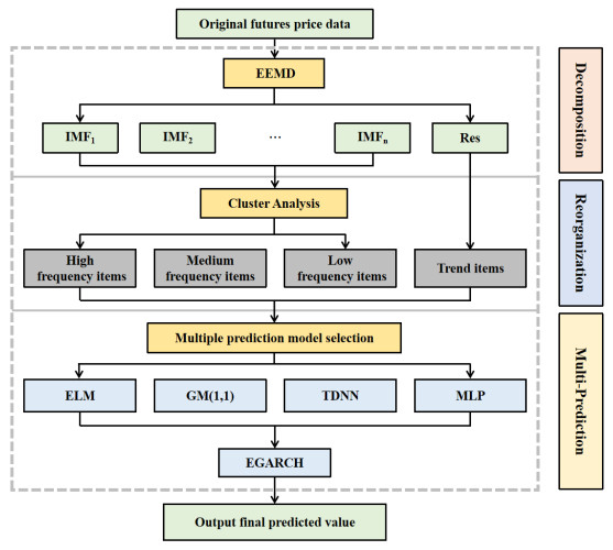
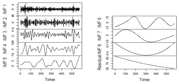
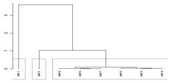
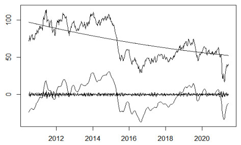
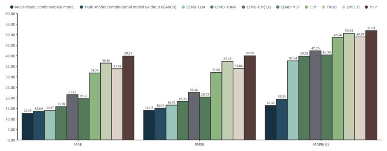
The crude oil market, as a complex evolutionary nonlinear driving system, is by nature a highly noisy, nonlinear and deterministic chaotic series of price series. In this paper, a computational intelligence-based portfolio model is constructed to forecast crude oil prices using weekly price data of West Texas intermediate crude oil (WTI) crude oil futures from 2011 to 2021. First, the WTI crude oil price series are decomposed using the ensemble empirical modal decomposition method (EEMD) and the set of component series is reconstructed using the cluster analysis method. Second, the reconstructed series are modeled and predicted using neural network models such as time-delay neural network (TDNN), extreme learning machine (ELM), multilayer perceptron (MLP) and the GM (1, 1) gray prediction algorithm and the output of the model with the best prediction effect for each component is integrated. Finally, the EGARCH model is used to further optimize the predictive power of the combined model and output the final predicted values. The results show that the combined model based on computational intelligence has higher forecasting accuracy than single models such as GM (1, 1), ARIMA, MLP and the combined EEMD-ELM model for forecasting crude oil futures prices.
Citation: Ming Li, Ying Li. Research on crude oil price forecasting based on computational intelligence[J]. Data Science in Finance and Economics, 2023, 3(3): 251-266. doi: 10.3934/DSFE.2023015
The crude oil market, as a complex evolutionary nonlinear driving system, is by nature a highly noisy, nonlinear and deterministic chaotic series of price series. In this paper, a computational intelligence-based portfolio model is constructed to forecast crude oil prices using weekly price data of West Texas intermediate crude oil (WTI) crude oil futures from 2011 to 2021. First, the WTI crude oil price series are decomposed using the ensemble empirical modal decomposition method (EEMD) and the set of component series is reconstructed using the cluster analysis method. Second, the reconstructed series are modeled and predicted using neural network models such as time-delay neural network (TDNN), extreme learning machine (ELM), multilayer perceptron (MLP) and the GM (1, 1) gray prediction algorithm and the output of the model with the best prediction effect for each component is integrated. Finally, the EGARCH model is used to further optimize the predictive power of the combined model and output the final predicted values. The results show that the combined model based on computational intelligence has higher forecasting accuracy than single models such as GM (1, 1), ARIMA, MLP and the combined EEMD-ELM model for forecasting crude oil futures prices.

| [1] |
Abdoos AA (2016) A new intelligent method based on combination of VMD and ELM for short term wind power forecasting. Neurocomputing 203: 111–120. https://doi.org/10.1016/j.neucom.2016.03.054 doi: 10.1016/j.neucom.2016.03.054

|
| [2] |
Akram QF (2020) Oil price drivers, geopolitical uncertainty and oil exporters' currencies. Energ Econo 89: 104801. https://doi.org/10.1016/j.eneco.2020.104801 doi: 10.1016/j.eneco.2020.104801
|
| [3] |
Baumeister C, Kilian L (2015) Forecasting the real price of oil in a changing world: a forecast combination approach. J Bu Econ Stat 33: 338–351. https://doi.org/10.1080/07350015.2014.949342 doi: 10.1080/07350015.2014.949342
|
| [4] |
Baumeister C, Kilian L (2016) Understanding the Decline in the Price of Oil since June 2014. J Assoc Enviro Resour Econ 3: 131–158. https://doi.org/10.1086/684160 doi: 10.1086/684160
|
| [5] |
Bouoiyour J, Selmi R, Hammoudeh S, et al. (2019) What are the categories of geopolitical risks that could drive oil prices higher? Acts or threats? Energ Econ 84: 104523. https://doi.org/10.1016/j.eneco.2019.104523 doi: 10.1016/j.eneco.2019.104523
|
| [6] |
Caldara D, Iacoviello M (2022) Measuring geopolitical risk. Am Econ Rev 112: 1194–1225. https://doi.org/10.1257/aer.20191823 doi: 10.1257/aer.20191823
|
| [7] |
Chen HH, Chen M, Chiu C C (2016) The integration of artificial neural networks and text mining to forecast gold futures prices. Commu Stat-Simul C 45: 1213–1225. https://doi.org/10.1080/03610918.2013.786780 doi: 10.1080/03610918.2013.786780
|
| [8] |
He M, Zhang Y, Wen D, et al. (2021) Forecasting crude oil prices: A scaled PCA approach. Energ Econ 97: 105189. https://doi.org/10.1016/j.eneco.2021.105189 doi: 10.1016/j.eneco.2021.105189
|
| [9] | Huifeng L (2017) Price forecasting of stock index futures based on a new hybrid EMD-RBF neural network model. Agro Food Ind Hi-Tech 28: 1744–1747. |
| [10] |
Morana C (2001) A semiparametric approach to short-term oil price forecasting. Energ Econ 23: 325–338. https://doi.org/10.1016/S0140-9883(00)00075-X doi: 10.1016/S0140-9883(00)00075-X
|
| [11] |
Phan DHB, Narayan PK, Gong Q (2021) Terrorist attacks and oil prices: Hypothesis and empirical evidence. Int Re Financ Anal 74: 101669. https://doi.org/10.1016/j.irfa.2021.101669 doi: 10.1016/j.irfa.2021.101669
|
| [12] |
Plourde A, Watkins GC (1998) Crude oil prices between 1985 and 1994: how volatile in relation to other commodities? Resour Energy Econ 20: 245–262. https://doi.org/10.1016/S0928-7655(97)00027-4 doi: 10.1016/S0928-7655(97)00027-4
|
| [13] | Tian LH, Tan DK (2015) Analysis of the factors influencing crude oil prices: financial speculation or Chinese demand? Economics (Quarterly) 14: 961–982. |
| [14] |
Wang C (2016) Forecast on price of agricultural futures in China based on ARIMA model. Asian Agric Res 8: 9. https://doi.org/10.22004/ag.econ.253255 doi: 10.22004/ag.econ.253255
|
| [15] |
Wu Z, Huang NE (2009) Ensemble empirical mode decomposition: a noise-assisted data analysis method. Adv Adapt Data Analysis 1: 1–41. https://doi.org/10.1142/S1793536909000047 doi: 10.1142/S1793536909000047
|
| [16] |
Yin L, Yang Q (2016) Predicting the oil prices: Do technical indicators help? Energ Econ 56: 338–350. https://doi.org/10.1016/j.eneco.2016.03.017 doi: 10.1016/j.eneco.2016.03.017
|
Figures(6) / Tables(3)
Ming Li, Ying Li. Research on crude oil price forecasting based on computational intelligence[J]. Data Science in Finance and Economics, 2023, 3(3): 251-266. doi: 10.3934/DSFE.2023015


 DownLoad: