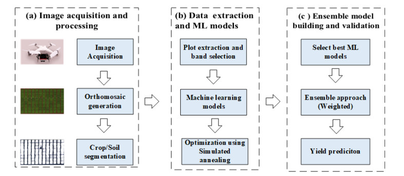
The unmanned aerial vehicle (UAV), as a remote sensing platform, has attracted many researchers in precision agriculture because of its operational flexibility and capability of producing high spatial and temporal resolution images of agricultural fields. This study proposed machine learning (ML) models and their ensembles for peanut yield prediction using UAV multispectral data. We utilized five bands (red, green, blue, near-infra-red (NIR) and red-edge) multispectral images acquired at various growth stages of peanuts using UAV. The correlation between spectral bands and yield was analyzed for each growth stage, which showed that the maturity stages had a significant correlation between peanut yield and spectral bands: red, green, NIR and red edge (REDE). Using these four bands spectral data, we assessed the potential for peanut yield prediction using multiple linear regression and seven non-linear ML models whose hyperparameters were optimized using simulated annealing (SA). The best three ML models, random forest (RF), support vector machine (SVM) and XGBoost, were then selected to construct a cooperative yield prediction framework with both the best ML model and the ensemble scheme from the best three as comparable recommendations to the farmers.
Citation: Tej Bahadur Shahi, Cheng-Yuan Xu, Arjun Neupane, Dayle B. Fleischfresser, Daniel J. O'Connor, Graeme C. Wright, William Guo. Peanut yield prediction with UAV multispectral imagery using a cooperative machine learning approach[J]. Electronic Research Archive, 2023, 31(6): 3343-3361. doi: 10.3934/era.2023169
The unmanned aerial vehicle (UAV), as a remote sensing platform, has attracted many researchers in precision agriculture because of its operational flexibility and capability of producing high spatial and temporal resolution images of agricultural fields. This study proposed machine learning (ML) models and their ensembles for peanut yield prediction using UAV multispectral data. We utilized five bands (red, green, blue, near-infra-red (NIR) and red-edge) multispectral images acquired at various growth stages of peanuts using UAV. The correlation between spectral bands and yield was analyzed for each growth stage, which showed that the maturity stages had a significant correlation between peanut yield and spectral bands: red, green, NIR and red edge (REDE). Using these four bands spectral data, we assessed the potential for peanut yield prediction using multiple linear regression and seven non-linear ML models whose hyperparameters were optimized using simulated annealing (SA). The best three ML models, random forest (RF), support vector machine (SVM) and XGBoost, were then selected to construct a cooperative yield prediction framework with both the best ML model and the ensemble scheme from the best three as comparable recommendations to the farmers.

| [1] | R. Nigam, R. Tripathy, S. Dutta, N. Bhagia, R. Nagori, K. Chandrasekar, et al., Crop type discrimination and health assessment using hyperspectral imaging, Curr. Sci., 116 (2019), 1108–1123. https://www.jstor.org/stable/27138003 |
| [2] |
J. ten Harkel, H. Bartholomeus, L. Kooistra, Biomass and crop height estimation of different crops using UAV-based LiDAR, Remote Sens., 12 (2020), 17. https://doi.org/10.3390/rs12010017 doi: 10.3390/rs12010017

|
| [3] |
U. S. Panday, N. Shrestha, S. Maharjan, A. K. Pratihast, Shahnawaz, K. L. Shrestha, et al., Correlating the plant height of wheat with above-ground biomass and crop yield using drone imagery and crop surface model, a case study from nepal, Drones, 4 (2020), 28. https://doi.org/10.3390/drones4030028 doi: 10.3390/drones4030028
|
| [4] |
A. Michez, P. Lejeune, S. Bauwens, A. A. L. Herinaina, Y. Blaise, E. C. Muñoz, et al., Mapping and monitoring of biomass and grazing in pasture with an unmanned aerial system, Remote Sens., 11 (2019), 473. https://doi.org/10.3390/rs11050473 doi: 10.3390/rs11050473
|
| [5] |
A. I. de Castro, R. Ehsani, R. C. Ploetz, J. H. Crane, S. Buchanon, Detection of laurel wilt disease in avocado using low altitude aerial imaging, PloS ONE, 10 (2015), 1–13. https://doi.org/10.1371/journal.pone.0124642 doi: 10.1371/journal.pone.0124642
|
| [6] |
A. Mahlein, Plant disease detection by imaging sensors–parallels and specific demands for precision agriculture and plant phenotyping, Plant Dis., 100 (2016), 241–251. https://doi.org/10.1094/PDIS-03-15-0340-FE doi: 10.1094/PDIS-03-15-0340-FE
|
| [7] | P. Moghadam, D. Ward, E. Goan, S. Jayawardena, P. Sikka, E. Hernandez, Plant disease detection using hyperspectral imaging, in 2017 International Conference on Digital Image Computing: Techniques and Applications (DICTA), (2017), 1–8. https://doi.org/10.1109/DICTA.2017.8227476 |
| [8] |
D. Gómez-Candón, J. Torres-Sanchez, S. Labbé, A. Jolivot, S. Martinez, J. L. Regnard, Water stress assessment at tree scale: high-resolution thermal UAV imagery acquisition and processing, Acta Hortic., 1150 (2017), 159–166. https://doi.org/10.17660/ActaHortic.2017.1150.23 doi: 10.17660/ActaHortic.2017.1150.23
|
| [9] |
C. A. Reynolds, M. Yitayew, D. C. Slack, C. F. Hutchinson, A. Huete, M. S. Petersen, Estimating crop yields and production by integrating the FAO Crop Specific Water Balance model with real-time satellite data and ground-based ancillary data, Int. J. Remote Sens., 21 (2000), 3487–3508. https://doi.org/10.1080/014311600750037516 doi: 10.1080/014311600750037516
|
| [10] |
S. S. Panda, D. P. Ames, S. Panigrahi, Application of vegetation indices for agricultural crop yield prediction using neural network techniques, Remote Sens., 2 (2010), 673–696. https://doi.org/10.3390/rs2030673 doi: 10.3390/rs2030673
|
| [11] |
Z. Fu, J. Jiang, Y. Gao, B. Krienke, M. Wang, K. Zhong, et al., Wheat growth monitoring and yield estimation based on multi-rotor unmanned aerial vehicle, Remote Sens., 12 (2020), 508. https://doi.org/10.3390/rs12030508 doi: 10.3390/rs12030508
|
| [12] |
S. Guan, K. Fukami, H. Matsunaka, M. Okami, R. Tanaka, H. Nakano, et al., Assessing correlation of high-resolution NDVI with fertilizer application level and yield of rice and wheat crops using small UAVs, Remote Sens., 11 (2019), 112. https://doi.org/10.3390/rs11020112 doi: 10.3390/rs11020112
|
| [13] |
M. Maimaitijiang, V. Sagan, P. Sidike, S. Hartling, F. Esposito, F. B. Fritschi, Soybean yield prediction from UAV using multimodal data fusion and deep learning, Remote Sens. Environ., 237 (2020), 111599. https://doi.org/10.1016/j.rse.2019.111599 doi: 10.1016/j.rse.2019.111599
|
| [14] |
Y. Guo, S. Chen, X. Li, M. Cunha, S. Jayavelu, D. Cammarano, et al., Machine learning-based approaches for predicting SPAD values of maize using multi-spectral images, Remote Sens., 14 (2022), 1337. https://doi.org/10.3390/rs14061337 doi: 10.3390/rs14061337
|
| [15] |
Z. Sun, X. Wang, Z. Wang, L. Yang, Y. Xie, Y. Huang, UAVs as remote sensing platforms in plant ecology: review of applications and challenges, J. Plant Ecol., 14 (2021), 1003–1023. https://doi.org/10.1093/jpe/rtab089 doi: 10.1093/jpe/rtab089
|
| [16] |
J. Xue, B. Su, Significant remote sensing vegetation indices: A review of developments and applications, J. Sens., 2017 (2017), 1–17. https://doi.org/10.1155/2017/1353691 doi: 10.1155/2017/1353691
|
| [17] |
L. Wan, H. Cen, J. Zhu, J. Zhang, Y. Zhu, D. Sun, et al., Grain yield prediction of rice using multi-temporal UAV-based RGB and multispectral images and model transfer-a case study of small farmlands in the South of China, Agric. For. Meteorol., 291 (2020), 108096. https://doi.org/10.1016/j.agrformet.2020.108096 doi: 10.1016/j.agrformet.2020.108096
|
| [18] |
J. Zhou, J. Zhou, H. Ye, M. L. Ali, P. Chen, H. T. Nguyen, Yield estimation of soybean breeding lines under drought stress using unmanned aerial vehicle-based imagery and convolutional neural network, Biosyst. Eng., 204 (2021), 90–103. https://doi.org/10.1016/j.biosystemseng.2021.01.017 doi: 10.1016/j.biosystemseng.2021.01.017
|
| [19] |
Y. Guo, H. Wang, Z. Wu, S. Wang, H. Sun, J. Senthilnath, et al., Modified red blue vegetation index for chlorophyll estimation and yield prediction of maize from visible images captured by UAV, Sensors, 20 (2020), 5055. https://doi.org/10.3390/s20185055 doi: 10.3390/s20185055
|
| [20] |
Y. Guo, Y. Fu, F. Hao, X. Zhang, W. Wu, X. Jin, et al., Integrated phenology and climate in rice yields prediction using machine learning methods, Ecol. Indic., 120 (2021), 106935. https://doi.org/10.1016/j.ecolind.2020.106935 doi: 10.1016/j.ecolind.2020.106935
|
| [21] | Peanut company of Australia, How peanuts are grown, 2023. Available from: https://pca.com.au/pca-profile/how-peanuts-are-grown/ |
| [22] |
Z. Ji, Y. Pan, X. Zhu, D. Zhang, J. Wang, A generalized model to predict large-scale crop yields integrating satellite-based vegetation index time series and phenology metrics, Ecol. Indic., 137 (2022), 108759. https://doi.org/10.1016/j.ecolind.2022.108759 doi: 10.1016/j.ecolind.2022.108759
|
| [23] |
H. García-Martínez, H. Flores-Magdaleno, R. Ascencio-Hernández, A. Khalil-Gardezi, L. Tijerina-Chávez, O. R. Mancilla-Villa, et al., Corn grain yield estimation from vegetation indices, canopy cover, plant density, and a neural network using multispectral and RGB images acquired with unmanned aerial vehicles, Agriculture, 10 (2020), 277. https://doi.org/10.3390/agriculture10070277 doi: 10.3390/agriculture10070277
|
| [24] |
X. Zhou, H. B. Zheng, X. Q. Xu, J. Y. He, X. K. Ge, X. Yao, et al., Predicting grain yield in rice using multi-temporal vegetation indices from UAV-based multispectral and digital imagery, ISPRS J. Photogramm. Remote Sens., 130 (2017), 246–255. https://doi.org/10.1016/j.isprsjprs.2017.05.003 doi: 10.1016/j.isprsjprs.2017.05.003
|
| [25] |
D. C. Tsouros, S. Bibi, P. G. Sarigiannidis, A review on UAV-based applications for precision agriculture, Information, 10 (2019), 349. https://doi.org/10.3390/info10110349 doi: 10.3390/info10110349
|
| [26] |
J. Kim, S. Kim, C. Ju, H. Il Son, Unmanned aerial vehicles in agriculture: A review of perspective of platform, control, and applications, IEEE Access, 7 (2019), 105100–105115. https://doi.org/10.1109/ACCESS.2019.2932119 doi: 10.1109/ACCESS.2019.2932119
|
| [27] |
T. B. Shahi, C. Xu, A. Neupane, W. Guo, Machine learning methods for precision agriculture with UAV imagery: A review, Electron. Res. Arch., 30 (2022), 4277–4317. https://doi.org/10.3934/era.2022218 doi: 10.3934/era.2022218
|
| [28] |
A. P. M. Ramos, L. P. Osco, D. E. G. Furuya, W. N. Gonçalves, D. C. Santana, L. P. R. Teodoro, et al., A random forest ranking approach to predict yield in maize with uav-based vegetation spectral indices, Comput. Electron. Agric., 178 (2020), 105791. https://doi.org/10.1016/j.compag.2020.105791 doi: 10.1016/j.compag.2020.105791
|
| [29] |
J. Geipel, J. Link, W. Claupein, Combined spectral and spatial modeling of corn yield based on aerial images and crop surface models acquired with an unmanned aircraft system, Remote sens., 6 (2014), 10335–10355. https://doi.org/10.3390/rs61110335 doi: 10.3390/rs61110335
|
| [30] | A. Ashapure, S. Oh, T. G. Marconi, A. Chang, J. Jung, J. Landivar, et al., Unmanned aerial system based tomato yield estimation using machine learning, in Autonomous Air and Ground Sensing Systems for Agricultural Optimization and Phenotyping IV, (2019). https://doi.org/10.1117/12.2519129 |
| [31] |
A. Matese, S. F. Di Gennaro, Beyond the traditional NDVI index as a key factor to mainstream the use of UAV in precision viticulture, Sci. Rep., 11 (2021), 1–13. https://doi.org/10.1038/s41598-021-81652-3 doi: 10.1038/s41598-021-81652-3
|
| [32] |
C. Bian, H. Shi, S. Wu, K. Zhang, M. Wei, Y. Zhao, et al., Prediction of field-scale wheat yield using machine learning method and multi-spectral UAV Ddata, Remote Sens., 14 (2022), 1474. https://doi.org/10.3390/rs14061474 doi: 10.3390/rs14061474
|
| [33] |
S. Fei, M. A. Hassan, Y. Xiao, X. Su, Z. Chen, Q. Cheng, et al., UAV-based multi-sensor data fusion and machine learning algorithm for yield prediction in wheat, Precision Agric., 24 (2022), 1–26. https://doi.org/10.1007/s11119-022-09938-8 doi: 10.1007/s11119-022-09938-8
|
| [34] |
A. Patrick, S. Pelham, A. Culbreath, C. C. Holbrook, I. J. De Godoy, C. Li, High throughput phenotyping of tomato spot wilt disease in peanuts using unmanned aerial systems and multispectral imaging, IEEE Instrum. Meas. Mag., 20 (2017), 4–12. https://doi.org/10.1109/MIM.2017.7951684 doi: 10.1109/MIM.2017.7951684
|
| [35] | QGIS development team, QGIS Geographic Information System, 2023. Available from: https://www.qgis.org |
| [36] |
F. I. Matias, M. V. Caraza-Harter, J. B. Endelman, FIELDimageR: An R package to analyze orthomosaic images from agricultural field trials, Plant Phenom. J., 3 (2020), 20005. https://doi.org/10.1002/ppj2.20005 doi: 10.1002/ppj2.20005
|
| [37] |
A. J. Smola, B. Schö lkopf, A tutorial on support vector regression, Satistics Comput., 14 (2004), 199–222. https://doi.org/10.1023/B:STCO.0000035301.49549.88 doi: 10.1023/B:STCO.0000035301.49549.88
|
| [38] |
X. Zeng, S. Yuan, Y. Li, Q. Zou, Decision tree classification model for popularity forecast of Chinese colleges, J. Appl. Math., (2014), 1–7. https://doi.org/10.1155/2014/675806 doi: 10.1155/2014/675806
|
| [39] |
L. Breiman, Random forests, Mach. Learn., 45 (2001), 5–32. https://doi.org/10.1023/A:1010933404324 doi: 10.1023/A:1010933404324
|
| [40] | F. Pedregosa, G. Varoquaux, A. Gramfort, V. Michel, B. Thirion, O. Grisel, et al., Scikit-learn: Machine learning in Python, J. Mach. Learn. Res., 12 (2011), 2825–2830. |
| [41] |
T. Hastie, S. Rosset, J. Zhu, H. Zou, Multi-class adaboost, Stat. Interface, 2 (2009), 349–360. https://doi.org/10.4310/SⅡ.2009.v2.n3.a8 doi: 10.4310/SⅡ.2009.v2.n3.a8
|
| [42] | T. Chen, C. Guestrin, Xgboost: A scalable tree boosting system, in Proceedings of the 22nd ACM SIGKDD International Conference on Knowledge Discovery and Data Mining, (2016), 785–794. https://doi.org/10.1145/2939672.2939785 |
| [43] |
M. M. Li, W. Guo, B. Verma, K. Tickle, J. O'Connor, Intelligent methods for solving inverse problems of backscattering spectra with noise: a comparison between neural networks and simulated annealing, Neural Comput. Appl., 18 (2009), 423–430. https://doi.org/10.1007/s00521-008-0219-x doi: 10.1007/s00521-008-0219-x
|
| [44] |
C. Tsai, C. Hsia, S. Yang, S. Liu, Z. Fang, Optimizing hyperparameters of deep learning in predicting bus passengers based on simulated annealing, Appl. Soft Comput., 88 (2020), 106068. https://doi.org/10.1016/j.asoc.2020.106068 doi: 10.1016/j.asoc.2020.106068
|
| [45] |
Q. Yan, J. Chen, L. De Strycker, An outlier detection method based on Mahalanobis distance for source localization, Sensors, 18 (2018), 2186. https://doi.org/10.3390/s18072186 doi: 10.3390/s18072186
|
| [46] |
B. Mishra, T. B. Shahi, Deep learning-based framework for spatiotemporal data fusion: an instance of landsat 8 and sentinel 2 NDVI, J. Appl. Remote Sens., 15 (2021), 034520. https://doi.org/10.1117/1.JRS.15.034520 doi: 10.1117/1.JRS.15.034520
|


Figures(5) / Tables(9)
Tej Bahadur Shahi, Cheng-Yuan Xu, Arjun Neupane, Dayle B. Fleischfresser, Daniel J. O'Connor, Graeme C. Wright, William Guo. Peanut yield prediction with UAV multispectral imagery using a cooperative machine learning approach[J]. Electronic Research Archive, 2023, 31(6): 3343-3361. doi: 10.3934/era.2023169


 DownLoad: