A network model of social contacts with small-world and scale-free features, tunable connectivity, and geographic restrictions

A. Newton Licciardi Jr.; L.H.A. Monteiro; A. Newton Licciardi Jr.; L.H.A. Monteiro

doi:10.3934/mbe.2024211

Mathematical Biosciences and Engineering

2024, Volume 21, Issue 4: 4801-4813. doi: 10.3934/mbe.2024211

Previous Article Next Article

Research article

A network model of social contacts with small-world and scale-free features, tunable connectivity, and geographic restrictions

A. Newton Licciardi Jr. ^1,2,
L.H.A. Monteiro ^{1,2
,
,}

1.
Universidade de São Paulo, Escola Politécnica, São Paulo, SP, Brazil
2.
Universidade Presbiteriana Mackenzie, Escola de Engenharia, São Paulo, SP, Brazil

Received: 08 October 2023 Revised: 10 December 2023 Accepted: 02 February 2024 Published: 29 February 2024

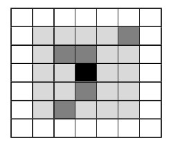
Small-world networks and scale-free networks are well-known theoretical models within the realm of complex graphs. These models exhibit "low" average shortest-path length; however, key distinctions are observed in their degree distributions and average clustering coefficients: in small-world networks, the degree distribution is bell-shaped and the clustering is "high"; in scale-free networks, the degree distribution follows a power law and the clustering is "low". Here, a model for generating scale-free graphs with "high" clustering is numerically explored, since these features are concurrently identified in networks representing social interactions. In this model, the values of average degree and exponent of the power-law degree distribution are both adjustable, and spatial limitations in the creation of links are taken into account. Several topological metrics are calculated and compared for computer-generated graphs. Unexpectedly, the numerical experiments show that, by varying the model parameters, a transition from a power-law to a bell-shaped degree distribution can occur. Also, in these graphs, the degree distribution is most accurately characterized by a pure power-law for values of the exponent typically found in real-world networks.
- complex network,
- power law,
- scale free,
- small world,
- social interaction
Citation: A. Newton Licciardi Jr., L.H.A. Monteiro. A network model of social contacts with small-world and scale-free features, tunable connectivity, and geographic restrictions[J]. Mathematical Biosciences and Engineering, 2024, 21(4): 4801-4813. doi: 10.3934/mbe.2024211

Related Papers:

Abstract

Small-world networks and scale-free networks are well-known theoretical models within the realm of complex graphs. These models exhibit "low" average shortest-path length; however, key distinctions are observed in their degree distributions and average clustering coefficients: in small-world networks, the degree distribution is bell-shaped and the clustering is "high"; in scale-free networks, the degree distribution follows a power law and the clustering is "low". Here, a model for generating scale-free graphs with "high" clustering is numerically explored, since these features are concurrently identified in networks representing social interactions. In this model, the values of average degree and exponent of the power-law degree distribution are both adjustable, and spatial limitations in the creation of links are taken into account. Several topological metrics are calculated and compared for computer-generated graphs. Unexpectedly, the numerical experiments show that, by varying the model parameters, a transition from a power-law to a bell-shaped degree distribution can occur. Also, in these graphs, the degree distribution is most accurately characterized by a pure power-law for values of the exponent typically found in real-world networks.

References

[1]	A. L. Barabási, R. Albert, H. Jeong, Scale-free characteristics of random networks: the topology of the World-Wide Web, Physica A, 281 (2000), 69–77. https://doi.org/10.1016/S0378-4371(00)00018-2 doi: 10.1016/S0378-4371(00)00018-2
[2]	R. Cohen, K. Erez, D. ben-Avraham, S. Havlin, Resilience of the Internet to random breakdowns, Phys. Rev. Lett., 85 (2000), 4626–4628. https://doi.org/10.1103/PhysRevLett.85.4626 doi: 10.1103/PhysRevLett.85.4626
[3]	H. A. Herrmann, J. M. Schwartz, Why COVID-19 models should incorporate the network of social interactions, Phys. Biol., 17 (2020), 065008. https://doi.org/10.1088/1478-3975/aba8ec doi: 10.1088/1478-3975/aba8ec
[4]	G. S. Hartnett, E. Parker, T. R. Gulden, R. Vardavas, D. Kravitz, Modelling the impact of social distancing and targeted vaccination on the spread of COVID-19 through a real city-scale contact network, J. Complex Netw., 9 (2021), cnab042. https://doi.org/10.1093/comnet/cnab042 doi: 10.1093/comnet/cnab042
[5]	D. Camacho, A. Panizo-LLedot, G. Bello-Orgaz, A. Gonzalez-Pardo, E. Cambria, The four dimensions of social network analysis: An overview of research methods, applications, and software tools, Inf. Fusion, 63 (2020), 88–120. https://doi.org/10.1016/j.inffus.2020.05.009 doi: 10.1016/j.inffus.2020.05.009
[6]	R. Pastor-Satorras, A. Vespignani, Epidemic spreading in scale-free networks, Phys. Rev. Lett., 86 (2001), 3200–3203. https://doi.org/10.1103/PhysRevLett.86.3200 doi: 10.1103/PhysRevLett.86.3200
[7]	D. Brockmann, D. Helbing, The hidden geometry of complex, network-driven contagion phenomena, Science, 342 (2013), 1337–1342. https://doi.org/10.1103/10.1126/science.1245200 doi: 10.1103/10.1126/science.1245200
[8]	E. N. Gilbert, Random graphs, Ann. Math. Statist., 30 (1959), 1141–1144. https://doi.org/10.1214/aoms/1177706098 doi: 10.1214/aoms/1177706098
[9]	P. Erdös, A. Rényi, On random graphs Ⅰ, Publ. Math. Debrecen, 6 (1959), 290–297.
[10]	P. Erdös, A. Rényi, On the evolution of random graphs, Publ. Math. Inst. Hungar. Acad. Sci., 5 (1960), 17–61.
[11]	R. Albert, A. L. Barabási, Statistical mechanics of complex networks, Rev. Mod. Phys., 74 (2002), 47–97. https://doi.org/10.1103/RevModPhys.74.47 doi: 10.1103/RevModPhys.74.47
[12]	M. E. J. Newman, The structure and function of complex networks, SIAM Rev., 45 (2003), 167–256. https://doi.org/10.1137/S003614450342480 doi: 10.1137/S003614450342480
[13]	S. Boccaletti, V. Latora, Y. Moreno, M. Chavez, D. U. Hwanga, Complex networks: Structure and dynamics, Phys. Rep., 424 (2006), 175–308. https://doi.org/10.1016/j.physrep.2005.10.009 doi: 10.1016/j.physrep.2005.10.009
[14]	F. Battiston, G. Cencetti, I. Iacopini, V. Latora, M. Lucas, A. Patania, et al., Networks beyond pairwise interactions: Structure and dynamics, Phys. Rep., 874 (2020), 1–92. https://doi.org/10.1016/j.physrep.2020.05.004 doi: 10.1016/j.physrep.2020.05.004
[15]	D. J. Watts, S. H. Strogatz, Collective dynamics of 'small-world' networks, Nature, 393 (1998), 440–442. https://doi.org/10.1038/30918 doi: 10.1038/30918
[16]	S. H. Strogatz, Exploring complex networks, Nature, 410 (2001), 268–276. https://doi.org/10.1038/35065725 doi: 10.1038/35065725
[17]	A. L. Barabási, R. Albert, Emergence of scaling in random networks, Science, 286 (1999), 509–512. https://doi.org/10.1126/science.286.5439.509 doi: 10.1126/science.286.5439.509
[18]	G. U. Yule, A mathematical theory of evolution, based on the conclusions of Dr. J. C. Willis, Philos. Trans. R. Soc. London Ser. B, 213 (1925), 21–87. https://doi.org/10.1098/rstb.1925.0002 doi: 10.1098/rstb.1925.0002
[19]	H. A. Simon, On a class of skew distribution functions, Biometrika, 42 (1955), 425–440. https://doi.org/10.1093/biomet/42.3-4.425 doi: 10.1093/biomet/42.3-4.425
[20]	D. J. S. Price, A general theory of bibliometric and other cumulative advantage processes, J. Amer. Soc. Inform. Sci., 27 (1976), 292–306. https://doi.org/10.1002/asi.4630270505 doi: 10.1002/asi.4630270505
[21]	G. Lima-Mendez, J. van Helden, The powerful law of the power law and other myths in network biology, Mol. Biosyst., 5 (2009), 1482–1493. https://doi.org/10.1039/b908681a doi: 10.1039/b908681a
[22]	W. Willinger, D. Alderson, J. C. Doyle, Mathematics and the Internet: A source of enormous confusion and great potential, Not. Am. Math. Soc., 56 (2009), 586–599.
[23]	A. D. Broido, A. Clauset, Scale-free networks are rare, Nat. Commun., 10 (2019), 1017. https://doi.org/10.1038/s41467-019-08746-5 doi: 10.1038/s41467-019-08746-5
[24]	C. Kasper, B. Voelkl, A social network analysis of primate groups, Primates, 50 (2009), 343–356. https://doi.org/10.1007/s10329-009-0153-2 doi: 10.1007/s10329-009-0153-2
[25]	S. Hennemann, B. Derudder, An alternative approach to the calculation and analysis of connectivity in the world city network, Environ. Plan. B-Plan. Des., 41 (2014), 392–412. https://doi.org/10.1068/b39108 doi: 10.1068/b39108
[26]	Y. L. Chuang, T. Chou, M. R. D'Orsogna, A network model of immigration: Enclave formation vs. cultural integration, Netw. Heterog. Media, 14 (2019), 53–77. https://doi.org/10.3934/nhm.2019004 doi: 10.3934/nhm.2019004
[27]	R. Munoz-Cancino, C. Bravo, S. A. Rios, M. Grana, On the combination of graph data for assessing thin-file borrowers' creditworthiness, Expert Syst. Appl., 213 (2023), 118809. https://doi.org/10.1016/j.eswa.2022.118809 doi: 10.1016/j.eswa.2022.118809
[28]	A. N. Licciardi Jr., L. H. A. Monteiro, A complex network model for a society with socioeconomic classes, Math. Biosci. Eng., 19 (2022), 6731–6742. https://doi.org/10.3934/mbe.2022317 doi: 10.3934/mbe.2022317
[29]	L. H. A. Monteiro, D. C. Paiva, J. R. C. Piqueira, Spreading depression in mainly locally connected cellular automaton, J. Biol. Syst., 14 (2006), 617–629. https://doi.org/10.1142/S0218339006001957 doi: 10.1142/S0218339006001957
[30]	P. H. T. Schimit, B. O. Santos, C. A. Soares, Evolution of cooperation in Axelrod tournament using cellular automata, Physica A, 437 (2015), 204–217. https://doi.org/10.1016/j.physa.2015.05.111 doi: 10.1016/j.physa.2015.05.111
[31]	P. H. T. Schimit, L. H. A. Monteiro, On the basic reproduction number and the topological properties of the contact network: An epidemiological study in mainly locally connected cellular automata, Ecol. Model., 220 (2009), 1034–1042. https://doi.org/10.1016/j.ecolmodel.2009.01.014 doi: 10.1016/j.ecolmodel.2009.01.014
[32]	H. A. L. R. Silva, L. H. A. Monteiro, Self-sustained oscillations in epidemic models with infective immigrants, Ecol. Complex., 17 (2014), 40–45. https://doi.org/10.1016/j.ecocom.2013.08.002 doi: 10.1016/j.ecocom.2013.08.002
[33]	L. H. A. Monteiro, D. M. Gandini, P. H. T. Schimit, The influence of immune individuals in disease spread evaluated by cellular automaton and genetic algorithm, Comput. Meth. Programs Biomed., 196 (2020), 105707. https://doi.org/10.1016/j.cmpb.2020.105707 doi: 10.1016/j.cmpb.2020.105707
[34]	K. Klemm, V. M. Eguiluz, Growing scale-free networks with small-world behavior, Phys. Rev. E, 65 (2002), 057102. https://doi.org/10.1103/PhysRevE.65.057102 doi: 10.1103/PhysRevE.65.057102
[35]	P. Holme, B. J. Kim, Growing scale-free networks with tunable clustering, Phys. Rev. E, 65 (2002), 026107. https://doi.org/10.1103/PhysRevE.65.026107 doi: 10.1103/PhysRevE.65.026107
[36]	Z. Z. Zhang, L. L. Rong, B. Wang, S. G. Zhou, J. H. Guan, Local-world evolving networks with tunable clustering, Physica A, 380 (2007), 639–650. https://doi.org/10.1016/j.physa.2007.02.045 doi: 10.1016/j.physa.2007.02.045
[37]	H. X. Yang, Z. X. Wu, W. B. Du, Evolutionary games on scale-free networks with tunable degree distribution, EPL, 99 (2012), 10006. https://doi.org/10.1209/0295-5075/99/10006 doi: 10.1209/0295-5075/99/10006
[38]	E. R. Colman, G. J. Rodgers, Complex scale-free networks with tunable power-law exponent and clustering, Physica A, 392 (2013), 5501–5510. https://doi.org/10.1016/j.physa.2013.06.063 doi: 10.1016/j.physa.2013.06.063
[39]	L. Wang, G. F. Li, Y. H. Ma, L. Yang, Structure properties of collaboration network with tunable clustering, Inf. Sci., 506 (2020), 37–50. https://doi.org/10.1016/j.ins.2019.08.002 doi: 10.1016/j.ins.2019.08.002
[40]	C. P. Warren, L. M. Sander, I. M. Sokolov, Geography in a scale-free network model, Phys. Rev. E, 66 (2002), 056105. https://doi.org/10.1103/PhysRevE.66.056105 doi: 10.1103/PhysRevE.66.056105
[41]	J. M. Kumpula, J. P. Onnela, J. Saramäki, K. Kaski, J. Kertész, Emergence of communities in weighted networks, Phys. Rev. Lett., 99 (2007), 228701. https://doi.org/10.1103/PhysRevLett.99.228701 doi: 10.1103/PhysRevLett.99.228701
[42]	Y. Murase, J. Török, H. H. Jo, K. Kaski, J. Kertész, Multilayer weighted social network model, Phys. Rev. E, 90 (2014), 052810. https://doi.org/10.1103/PhysRevE.90.052810 doi: 10.1103/PhysRevE.90.052810
[43]	S. Wolfram, Cellular automata and complexity: Collected papers, Westview Press, Boulder, 1994.
[44]	A. Landherr, B. Friedl, J. Heidemann, A critical review of centrality measures in social networks, Bus. Inf. Syst. Eng., 2 (2010), 371–385. https://doi.org/10.1007/s12599-010-0127-3 doi: 10.1007/s12599-010-0127-3
[45]	L. Ljung, System identification: Theory for the user, Prentice-Hall, Upper Saddle River, 1998.
[46]	A. Clauset, C. R. Shalizi, M. E. J. Newman, Power-law distributions in empirical data, SIAM Rev., 51 (2009), 661–703. https://doi.org/10.1137/070710111 doi: 10.1137/070710111
[47]	F. Liljeros, C. R. Edling, L. A. N. Amaral, H. E. Stanley, Y. Aberg, The web of human sexual contacts, Nature, 411 (2001), 907–908. https://doi.org/10.1038/35082140 doi: 10.1038/35082140

Reader Comments

Your name:*

Email:*
© 2024 the Author(s), licensee AIMS Press. This is an open access article distributed under the terms of the Creative Commons Attribution License (http://creativecommons.org/licenses/by/4.0)