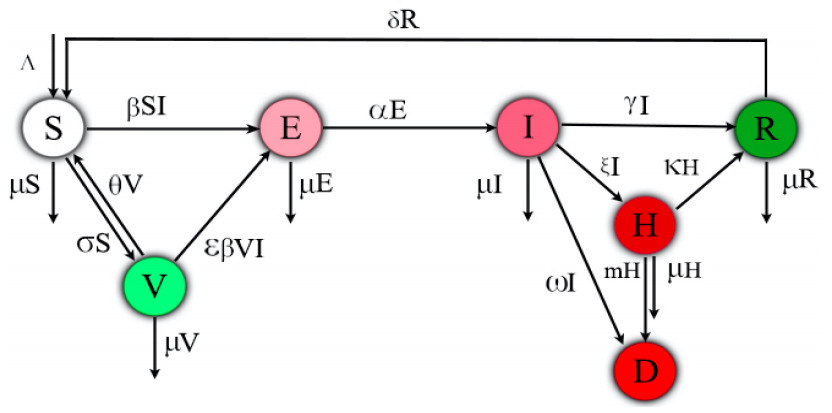
This paper is devoted to investigating the impact of vaccination on mitigating COVID-19 outbreaks. In this work, we propose a compartmental epidemic ordinary differential equation model, which extends the previous so-called SEIRD model [
Citation: Allison Fisher, Hainan Xu, Daihai He, Xueying Wang. Effects of vaccination on mitigating COVID-19 outbreaks: a conceptual modeling approach[J]. Mathematical Biosciences and Engineering, 2023, 20(3): 4816-4837. doi: 10.3934/mbe.2023223
This paper is devoted to investigating the impact of vaccination on mitigating COVID-19 outbreaks. In this work, we propose a compartmental epidemic ordinary differential equation model, which extends the previous so-called SEIRD model [

| [1] | H. Song, G. Fan, Y. Liu, X. Wang, D. He, The second wave of COVID-19 in South and Southeast Asia and the effects of vaccination, Front. Med., 8 (2021). https://doi.org/10.3389/fmed.2021.773110 |
| [2] |
H. Song, G. Fan, S. Zhao, H. Li, Q. Huang, D. He, Forecast of the COVID-19 trend in India: a simple modelling approach, Math. Biosci. Eng., 8 (2021), 9775–9786. https://doi.org/10.3934/mbe.2021479 doi: 10.3934/mbe.2021479

|
| [3] | S. S. Musa, A. Tariq, L. Yuan, W. Haozhen, D. He, Infection fatality rate and infection attack rate of COVID-19 in South American countries, Infect. Dis. Poverty, 11 (2022). https://doi.org/10.1186/s40249-022-00961-5 |
| [4] | S. S. Musa, X. Wang, S. Zhao, S. Li, N. Hussaini, W. Wang, et al., The heterogeneous severity of COVID-19 in African countries: a modeling approach, Bull. Math. Biol., 84 (2022), 1–16. Available from: https://link.springer.com/article/10.1007/s11538-022-00992-x. |
| [5] |
G. B. Libotte, F. S. Lobato, G. M. Platt, A. J. S. Neto, Determination of an optimal control strategy for vaccine administration in COVID-19 pandemic treatment, Comput. Methods Programs Biomed., 196 (2020), 105664. https://doi.org/10.1016/j.cmpb.2020.105664 doi: 10.1016/j.cmpb.2020.105664
|
| [6] |
C. M. Saad-Roy, S. E. Morris, C. J. E. Metcalf, M. J. Mina, R. E. Baker, J. Farrar, et al., Epidemiological and evolutionary considerations of SARS-CoV-2 vaccine dosing regimes, Science, 372 (2021), 363–370. https://doi.org/10.1126/science.abg8663 doi: 10.1126/science.abg8663
|
| [7] |
M. Makhoul, H. H. Ayoub, H. Chemaitelly, S. Seedat, G. R. Mumtaz, S. Al-Omari, et al., Epidemiological impact of SARS-CoV-2 vaccination: mathematical modeling analyses, Vaccines, 8 (2020), 668. https://doi.org/10.3390/vaccines8040668 doi: 10.3390/vaccines8040668
|
| [8] | S. Berkane, I. Harizi, A. Tayebi, Modeling the effect of population-wide vaccination on the evolution of COVID-19 epidemic in Canada, medRxiv preprint, 2021. https://doi.org/10.1101/2021.02.05.21250572 |
| [9] |
N. P. Rachaniotis, T. K. Dasaklis, F. Fotopoulos, P. Tinios, A two-phase stochastic dynamic model for COVID-19 mid-term policy recommendations in Greece: a pathway towards mass vaccination, Int. J. Environ. Res. Public Health, 18 (2021), 2497. https://doi.org/10.3390/ijerph18052497 doi: 10.3390/ijerph18052497
|
| [10] |
E. Shim, Optimal allocation of the limited COVID-19 vaccine supply in South Korea, J. Clin. Med., 10 (2021), 591. https://doi.org/10.3390/jcm10040591 doi: 10.3390/jcm10040591
|
| [11] |
E. Shim, Projecting the impact of SARS-CoV-2 variants and the vaccination program on the fourth wave of the COVID-19 pandemic in South Korea, Int. J. Environ. Res. Public Health, 18 (2021), 7578. https://doi.org/10.3390/ijerph18147578 doi: 10.3390/ijerph18147578
|
| [12] |
G. Webb, A COVID-19 epidemic model predicting the effectiveness of vaccination in the US, Infect. Dis. Rep., 13 (2021), 654–667. https://doi.org/10.3390/idr13030062 doi: 10.3390/idr13030062
|
| [13] |
S. Roy, R. Dutta, P. Ghosh, Optimal time-varying vaccine allocation amid pandemics with uncertain immunity ratios, IEEE Access, 9 (2021), 15110–15121. https://doi.org/10.1109/ACCESS.2021.3053268 doi: 10.1109/ACCESS.2021.3053268
|
| [14] |
F. Amaral, W. Casaca, C. M. Oishi, J. A. Cuminato, Simulating immunization campaigns and vaccine protection against COVID-19 pandemic in Brazil, IEEE Access, 9 (2021), 126011–126022. https://doi.org/10.1109/ACCESS.2021.3112036 doi: 10.1109/ACCESS.2021.3112036
|
| [15] |
M. Etxeberria-Etxaniz, S. Alonso-Quesada, M. De la Sen, On an SEIR epidemic model with vaccination of newborns and periodic impulsive vaccination with eventual on-line adapted vaccination strategies to the varying levels of the susceptible subpopulation, Appl. Sci., 10 (2020), 8296. https://doi.org/10.3390/app10228296 doi: 10.3390/app10228296
|
| [16] |
S. M. Moghadas, T. N. Vilches, K. Zhang, C. R. Wells, A. Shoukat, B. H. Singer, et al., The impact of vaccination on coronavirus disease 2019 (COVID-19) outbreaks in the United States, Clin. Infect. Dis., 73 (2021), 2257–2264. https://doi.org/10.1093/cid/ciab079 doi: 10.1093/cid/ciab079
|
| [17] |
L. Lin, Y. Zhao, B. Chen, D. He, Multiple COVID-19 waves and vaccination effectiveness in the United States, Int. J. Environ. Res. Public Health, 19 (2022), 2282. https://doi.org/10.3390/ijerph19042282 doi: 10.3390/ijerph19042282
|
| [18] |
F. T. Goh, Y. Z. Chew, C. C. Tam, C. F. Yung, H. Clapham, A country-specific model of COVID-19 vaccination coverage needed for herd immunity in adult only or population wide vaccination programme, Epidemics, 39 (2022), 100581. https://doi.org/10.1016/j.epidem.2022.100581 doi: 10.1016/j.epidem.2022.100581
|
| [19] | D. McEvoy, C. McAloon, A. Collins, K. Hunt, F. Butler, A. Byrne, et al., Relative infectiousness of asymptomatic SARS-CoV-2 infected persons compared with symptomatic individuals: a rapid scoping review, BMJ Open, 11 (2021), e042354. |
| [20] |
B. K. Singh, J. Walker, P. Paul, S. Reddy, B. K. Gowler, J. Jernigan, et al., De-escalation of asymptomatic testing and potential of future COVID-19 outbreaks in US nursing homes amidst rising community vaccination coverage: a modeling study, Vaccine, 40 (2022), 3165–3173. https://doi.org/10.1016/j.vaccine.2022.04.040 doi: 10.1016/j.vaccine.2022.04.040
|
| [21] |
Y. Goldberg, M. Mandel, Y. M. Bar-On, O. Bodenheimer, L. Freedman, E. J. Haas, et al., Waning immunity after the BNT162b2 vaccine in Israel, N. Engl. J. Med., 385 (2021), e85. https://doi.org/10.1056/NEJMoa2114228 doi: 10.1056/NEJMoa2114228
|
| [22] |
W. Yang, J. Shaman, Development of a model-inference system for estimating epidemiological characteristics of SARS-CoV-2 variants of concern, Nat. Commun., 12 (2021), 1–9. https://doi.org/10.1038/s41467-021-25913-9 doi: 10.1038/s41467-021-25913-9
|
| [23] |
G. Fan, H. Song, S. Yip, T. Zhang, D. He, Impact of low vaccine coverage on the resurgence of COVID-19 in Central and Eastern Europe, One Health, 14 (2022), 100402. https://doi.org/10.1016/j.onehlt.2022.100402 doi: 10.1016/j.onehlt.2022.100402
|
| [24] |
J. S. Lavine, O. N. Bjornstad, R. Antia, Immunological characteristics govern the transition of COVID-19 to endemicity, Science, 371 (2021), 741–745. https://doi.org/10.1126/science.abe6522 doi: 10.1126/science.abe6522
|
| [25] |
X. Tang, S. S. Musa, S. Zhao, S. Mei, D. He, Using proper mean generation intervals in modeling of COVID-19, Front. Public Health, 9 (2021), 691262. https://doi.org/10.3389/fpubh.2021.691262 doi: 10.3389/fpubh.2021.691262
|
| [26] |
Y. Liu, K. Wang, L. Yang, D. He, Regional heterogeneity of in-hospital mortality of COVID-19 in Brazil, Infect. Dis. Modell., 7 (2022), 364–373. https://doi.org/10.1016/j.idm.2022.06.005 doi: 10.1016/j.idm.2022.06.005
|
| [27] | X. Q. Zhao, Dynamical Systems in Population Biology, 2$^{nd}$ edition, Springer, Cham, 2017. |
| [28] | X. Q. Zhao, Asymptotic behavior for asymptotically periodic semiflows with applications, 1996. |
| [29] | N. Bacaër, S. Guernaoui, The epidemic threshold of vector-borne diseases with seasonality, J. Math. Biol., 53 (2006), 421–436. |
| [30] |
J. M. Heffernan, R. J. Smith, L. M. Wahl, Perspectives on the basic reproductive ratio, J. R. Soc. Interface, 2 (2005), 281–293. https://doi.org/10.1098/rsif.2005.0042 doi: 10.1098/rsif.2005.0042
|
| [31] |
H. R. Thieme, Spectral bound and reproduction number for infinite-dimensional population structure and time heterogeneity, SIAM J. Appl. Math., 70 (2009), 188–211. https://doi.org/10.1137/080732870 doi: 10.1137/080732870
|
| [32] |
W. Wang, X. Q. Zhao, Threshold dynamics for compartmental epidemic models in periodic environments, J. Dyn. Differ. Equations, 20 (2008), 699–717. https://doi.org/10.1007/s10884-008-9111-8 doi: 10.1007/s10884-008-9111-8
|
| [33] |
X. Q. Zhao, Basic reproduction ratios for periodic compartmental models with time delay, J. Dyn. Differ. Equations, 29 (2017), 67–82. https://doi.org/10.1007/s10884-015-9425-2 doi: 10.1007/s10884-015-9425-2
|
| [34] |
G. Aronsson, R. B. Kellogg, On a differential equation arising from compartmental analysis, Math. Biosci., 38 (1978), 113–122. https://doi.org/10.1016/0025-5564(78)90021-4 doi: 10.1016/0025-5564(78)90021-4
|
| [35] |
M. W. Hirsch, Systems of differential equations that are competitive or cooperative II: convergence almost everywhere, SIAM J. Math. Anal., 16 (1985), 423–439. https://doi.org/10.1137/0516030 doi: 10.1137/0516030
|
| [36] |
F. Zhang, X. Q. Zhao, A periodic epidemic model in a patchy environment, J. Math. Anal. Appl., 325 (2007), 496–516. https://doi.org/10.1016/j.jmaa.2006.01.085 doi: 10.1016/j.jmaa.2006.01.085
|
| [37] | H. L. Smith, Monotone Dynamical Systems: an Introduction to the Theory of Competitive and Cooperative Systems, American Mathematical Society, 2008. |
| [38] | E. Mathieu, H. Ritchie, E. Ortiz-Ospina, M. Roser, J. Hasell, C. Appel, et al., A global database of COVID-19 vaccinations, Nat. Hum. Behav., 5 (2021), 947–953. |
| [39] | Owid, Dataset, 2022. Available from: https://covid.ourworldindata.org. |
| [40] |
L. Lin, B. Chen, Y. Zhao, W. Wang, D. He, Two waves of COVID-19 in Brazilian cities and vaccination impact, Math. Biosci. Eng., 19 (2021), 4657–4671. http://dx.doi.org/10.2139/ssrn.3977464 doi: 10.2139/ssrn.3977464
|
| [41] |
E. L. Ionides, C. Breto, A. A. King, Inference for nonlinear dynamical systems, Proc. Natl. Acad. Sci. U.S.A., 103 (2006), 18438–18443. https://doi.org/10.1073/pnas.0603181103 doi: 10.1073/pnas.0603181103
|
| [42] |
S. S. Musa, S. Zhao, D. Gao, Q. Lin, G. Chowell, D. He, Mechanistic modelling of the large-scale Lassa fever epidemics in Nigeria from 2016 to 2019, J. Theor. Biol., 493 (2020), 110209. https://doi.org/10.1016/j.jtbi.2020.110209 doi: 10.1016/j.jtbi.2020.110209
|
| [43] | C. Breto, D. He, E. L. Ionides, A. A. King, Time series analysis via mechanistic models, Ann. Appl. Stat., 3 (2009), 319–348. Available from: https://www.jstor.org/stable/30244243. |
| [44] | D. He, S. T. Ali, G. Fan, D. Gao, H. Song, Y. Lou, et al., Evaluation of effectiveness of global COVID-19 vaccination campaign, Emerging Infect. Dis., 28 (2022), 1873–1876. |
| [45] |
D. He, S. Zhao, Q. Lin, S. S. Musa, L. Stone, New estimates of the Zika virus epidemic attack rate in Northeastern Brazil from 2015 to 2016: a modelling analysis based on Guillain-Barré Syndrome (GBS) surveillance data, PLoS Negl. Trop. Dis., 14 (2020), e0007502. https://doi.org/10.1371/journal.pntd.0007502 doi: 10.1371/journal.pntd.0007502
|
| [46] | L. Stone, D. He, S. Lehnstaedt, Y. Artzy-Randrup, Extraordinary curtailment of massive typhus epidemic in the Warsaw Ghetto, Sci. Adv., 6 (2020). https://doi.org/10.1126/sciadv.abc0927 |
| [47] |
S. Zhao, L. Stone, D. Gao, D. He, Modelling the large-scale yellow fever outbreak in Luanda, Angola, and the impact of vaccination, PLoS Negl. Trop. Dis., 12 (2021), e0006158. https://doi.org/10.1371/journal.pntd.0006158 doi: 10.1371/journal.pntd.0006158
|
| [48] | Simulation-based inference for epidemiological dynamics. Available from: https://kingaa.github.io/sbied/ |
| [49] | A. A. King, E. L. Ionides, M. Pascual, M. J. Bouma, Inapparent infections and cholera dynamics, Nature, 454 (2008), 877–880. |


Figures(5) / Tables(1)

Allison Fisher, Hainan Xu, Daihai He, Xueying Wang. Effects of vaccination on mitigating COVID-19 outbreaks: a conceptual modeling approach[J]. Mathematical Biosciences and Engineering, 2023, 20(3): 4816-4837. doi: 10.3934/mbe.2023223


 DownLoad: