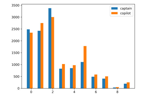
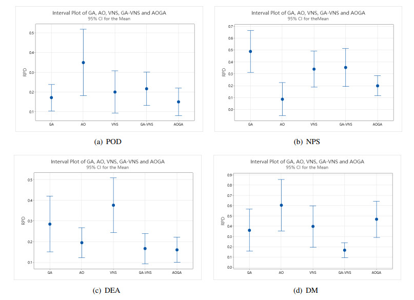
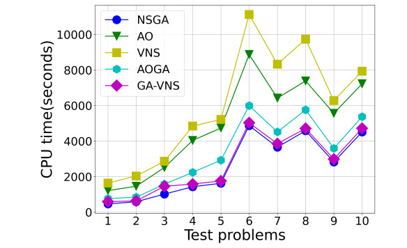
In order to cope with the rapid growth of flights and limited crew members, the rational allocation of crew members is a strategy to greatly alleviate scarcity. However, if there is no appropriate allocation plan, some flights may be canceled because there is no pilot in the scheduling period. In this paper, we solved an airline crew rostering problem (CRP). We model the CRP as an integer programming model with multiple constraints and objectives. In this model, the schedule of pilots takes into account qualification restrictions and language restrictions, while maximizing the fairness and satisfaction of pilots. We propose the design of two hybrid metaheuristic algorithms based on a genetic algorithm, variable neighborhood search algorithm and the Aquila optimizer to face the trade-off between fairness and crew satisfaction. The simulation results show that our approach preserves the fairness of the system and maximizes the fairness at the cost of crew satisfaction.
Citation: Bin Deng, Ran Ding, Jingfeng Li, Junfeng Huang, Kaiyi Tang, Weidong Li. Hybrid multi-objective metaheuristic algorithms for solving airline crew rostering problem with qualification and language[J]. Mathematical Biosciences and Engineering, 2023, 20(1): 1460-1487. doi: 10.3934/mbe.2023066
In order to cope with the rapid growth of flights and limited crew members, the rational allocation of crew members is a strategy to greatly alleviate scarcity. However, if there is no appropriate allocation plan, some flights may be canceled because there is no pilot in the scheduling period. In this paper, we solved an airline crew rostering problem (CRP). We model the CRP as an integer programming model with multiple constraints and objectives. In this model, the schedule of pilots takes into account qualification restrictions and language restrictions, while maximizing the fairness and satisfaction of pilots. We propose the design of two hybrid metaheuristic algorithms based on a genetic algorithm, variable neighborhood search algorithm and the Aquila optimizer to face the trade-off between fairness and crew satisfaction. The simulation results show that our approach preserves the fairness of the system and maximizes the fairness at the cost of crew satisfaction.

| [1] | Civil Aviation Administration of China, 2018 Civil Aviation Industry Development Statistics Bulletin, 2019. Available from: http://www.caac.gov.cn/XXGK/XXGK/TJSJ/201905/P0201905085195 29727887.pdf. |
| [2] |
M. Ehrgott, D. M. Ryan, Constructing robust crew schedules with bicriteria optimization, J. Multi-Criter. Decis. Anal., 11 (2002), 139–150. https://doi.org/10.1002/mcda.321 doi: 10.1002/mcda.321

|
| [3] |
S. Zhou, Z. Zhan, Z. Chen, S. Kwong, J. Zhang, A multi-objective ant colony system algorithm for airline crew rostering problem with fairness and satisfaction, IEEE Trans. Intell. Transp. Syst., 22 (2020), 6784–6798. https://doi.org/10.1109/TITS.2020.2994779 doi: 10.1109/TITS.2020.2994779
|
| [4] |
R. T. Marler, J. S. Arora, Survey of multi-objective optimization methods for engineering, Struct. Multidiscip. Optim., 26 (2004), 369–395. https://doi.org/10.1007/s00158-003-0368-6 doi: 10.1007/s00158-003-0368-6
|
| [5] |
Q. Yang, L. Dan, M. Lv, J. Wu, W. Li, W. Dong, Quantitative assessment of the parameterization sensitivity of the Noah-MP land surface model with dynamic vegetation using ChinaFLUX data, Agric. For. Meteorol., 307 (2021), 108542. https://doi.org/10.1016/j.agrformet.2021.108542 doi: 10.1016/j.agrformet.2021.108542
|
| [6] |
Q. Yang, L. Dan, J. Wu, R. Jiang, J. Dan, W. Li, et al., The improved freeze–thaw process of a climate-vegetation model: Calibration and validation tests in the source region of the Yellow River, Agric. For. Meteorol., 123 (2018), 346–367. https://doi.org/10.1029/2017JD028050 doi: 10.1029/2017JD028050
|
| [7] |
J. E. Beasley, B. Cao, A tree search algorithm for the crew scheduling problem, Eur. J. Oper. Res., 94 (1996), 517–526. https://doi.org/10.1016/0377-2217(95)00093-3 doi: 10.1016/0377-2217(95)00093-3
|
| [8] |
J. E. Beasley, B. Cao, A dynamic programming based algorithm for the crew scheduling problem, Comput. Oper. Res., 25 (1998), 567–582. https://doi.org/10.1016/S0305-0548(98)00019-7 doi: 10.1016/S0305-0548(98)00019-7
|
| [9] |
P. Lučić, D. Teodorović, Metaheuristics approach to the aircrew rostering problem, Ann. Oper. Res., 155 (2007), 311–338. https://doi.org/10.1007/s10479-007-0216-y doi: 10.1007/s10479-007-0216-y
|
| [10] |
B. Maenhout, M. Vanhoucke, A hybrid scatter search heuristic for personalized crew rostering in the airline industry, Eur. J. Oper. Res., 206 (2010), 155–167. https://doi.org/10.1016/j.ejor.2010.01.040 doi: 10.1016/j.ejor.2010.01.040
|
| [11] |
R. Hadianti, K. Novianingsih, S. Uttunggadewa, K. Sidarto, N. Sumarti, E. Soewono, Optimization model for an airline crew rostering problem: Case of Garuda Indonesia, J. Math. Fundam. Sci., 45 (2013), 218–234. https://doi.org/10.5614/j.math.fund.sci.2013.45.3.2 doi: 10.5614/j.math.fund.sci.2013.45.3.2
|
| [12] |
F. Quesnel, G. Desaulniers, F. Soumis, Improving air crew rostering by considering crew preferences in the crew pairing problem, Transp. Sci., 54 (2020), 97–114. https://doi.org/10.1287/trsc.2019.0913 doi: 10.1287/trsc.2019.0913
|
| [13] |
F. Quesnel, A. Wu, G. Desaulniers, F. Soumis, Deep-learning-based partial pricing in a branch-and-price algorithm for personalized crew rostering, Comput. Oper. Res., 138 (2022), 105554. https://doi.org/10.1016/j.cor.2021.105554 doi: 10.1016/j.cor.2021.105554
|
| [14] |
B. Deng, An improved honey badger algorithm by genetic algorithm and levy flight distribution for solving airline crew rostering problem, IEEE Access, 10 (2022), 108075–108088. https://doi.org/10.1109/ACCESS.2022.3213066 doi: 10.1109/ACCESS.2022.3213066
|
| [15] |
N. Souai, J. Teghem, Genetic algorithm based approach for the integrated airline crew-pairing and rostering problem, Eur. J. Oper. Res., 199 (2009), 674–683. https://doi.org/10.1016/j.ejor.2007.10.065 doi: 10.1016/j.ejor.2007.10.065
|
| [16] |
M. Saddoune, G. Desaulniers, I. Elhallaoui, F. Soumis, A. Fathollahi-Fard, Integrated airline crew pairing and crew assignment by dynamic constraint aggregation, Transp. Sci., 46 (2012), 39–55. https://doi.org/10.1287/trsc.1110.0379 doi: 10.1287/trsc.1110.0379
|
| [17] |
V. Zeighami, M. Saddoune, F. Soumis, Alternating Lagrangian decomposition for integrated airline crew scheduling problem, Eur. J. Oper. Res., 287 (2020), 211–224. https://doi.org/10.1016/j.ejor.2020.05.005 doi: 10.1016/j.ejor.2020.05.005
|
| [18] |
A. M. Fathollahi-Fard, A. Ahmadi, F. Goodarzian, N. Cheikhrouhou, A bi-objective home healthcare routing and scheduling problem considering patients' satisfaction in a fuzzy environment, Appl. Soft Comput., 93 (2020), 106385. https://doi.org/10.1016/j.asoc.2020.106385 doi: 10.1016/j.asoc.2020.106385
|
| [19] |
Z. Sazvar, S. Mirzapour Al-E-Hashem, A. Baboli, M. A. Jokar, A bi-objective stochastic programming model for a centralized green supply chain with deteriorating products, Int. J. Prod. Econ., 150 (2014), 140–154. https://doi.org/10.1016/j.ijpe.2013.12.023 doi: 10.1016/j.ijpe.2013.12.023
|
| [20] |
J. Pasha, A. L. Nwodu, A. M. Fathollahi-Fard, G. Tian, Z. Li, H. Wang, et al., Exact and metaheuristic algorithms for the vehicle routing problem with a factory-in-a-box in multi-objective settings, Adv. Eng. Inf., 52 (2022), 101623. https://doi.org/10.1016/j.aei.2022.101623 doi: 10.1016/j.aei.2022.101623
|
| [21] |
A. M. Fathollahi-Fard, L. Woodward, O. Akhrif, Sustainable distributed permutation flow-shop scheduling model based on a triple bottom line concept, J. Ind. Inf. Integr., 24 (2021), 100233. https://doi.org/10.1016/j.jii.2021.100233 doi: 10.1016/j.jii.2021.100233
|
| [22] |
E. K. Burke, P. De Causmaecker, G. De Maere, J. Mulder, M. Paelinck, G. V. Berghe, A multi-objective approach for robust airline scheduling, Comput. Oper. Res., 37 (2010), 822–832. https://doi.org/10.1016/j.cor.2009.03.026 doi: 10.1016/j.cor.2009.03.026
|
| [23] |
P. Chutima, K. Arayikanon, Many-objective low-cost airline cockpit crew rostering optimisation, Comput. Ind. Eng., 150 (2020), 106844. https://doi.org/10.1016/j.cie.2020.106844 doi: 10.1016/j.cie.2020.106844
|
| [24] |
V. Baradaran, A. H. Hosseinian, A multi-objective mathematical formulation for the airline crew scheduling problem: MODE and NSGA-II solution approaches, J. Ind. Manage. Perspect., 11 (2021), 247–269. https://doi.org/10.52547/jimp.11.1.247 doi: 10.52547/jimp.11.1.247
|
| [25] |
Q. Yang, H. Zuo, W. Li, Land surface model and particle swarm optimization algorithm based on the model-optimization method for improving soil moisture simulation in a semi-arid region, Plos One, 11 (2016), e0151576. https://doi.org/10.1371/journal.pone.0151576 doi: 10.1371/journal.pone.0151576
|
| [26] |
Q. Yang, J. Wu, Y. Li, W. Li, L. Wang, Y. Yang, Using the particle swarm optimization algorithm to calibrate the parameters relating to the turbulent flux in the surface layer in the source region of the Yellow River, Agric. For. Meteorol., 232 (2017), 606–622. https://doi.org/10.1016/j.agrformet.2016.10.019 doi: 10.1016/j.agrformet.2016.10.019
|
| [27] |
L. Abualigah, D. Yousri, M. A. Al-Qaness, A. H. Gandomi, Aquila optimizer: A novel meta-heuristic optimization algorithm, Comput. Ind. Eng., 157 (2021), 107250. https://doi.org/10.1016/j.cie.2021.107250 doi: 10.1016/j.cie.2021.107250
|
| [28] |
B. Naderi, R. Tavakkoli-Moghaddam, M. Khalili, Electromagnetism-like mechanism and simulated annealing algorithms for flowshop scheduling problems minimizing the total weighted tardiness and makespan, Knowl. Based Syst., 23 (2010), 77–85. https://doi.org/10.1016/j.knosys.2009.06.002 doi: 10.1016/j.knosys.2009.06.002
|
| [29] |
B. Vahdani, M. Zandieh, Scheduling trucks in cross-docking systems: Robust meta-heuristics, Comput. Ind. Eng., 58 (2010), 12–24. https://doi.org/10.1016/j.cie.2009.06.006 doi: 10.1016/j.cie.2009.06.006
|
| [30] |
M. Abd Elaziz, A. Dahou, N. A. Alsaleh, A. H. Elsheikh, A. I. Saba, M. Ahmadein, Boosting COVID-19 image classification using MobileNetV3 and aquila optimizer algorithm, Entropy, 23 (2021), 1383. https://doi.org/10.3390/e23111383 doi: 10.3390/e23111383
|
| [31] |
A. M. AlRassas, M. A. Al-qaness, A. A. Ewees, S. Ren, M. Abd Elaziz, R. Damaševičius, et al., Optimized ANFIS model using Aquila Optimizer for oil production forecasting, Processes, 9 (2021), 1194. https://doi.org/10.3390/pr9071194 doi: 10.3390/pr9071194
|
| [32] |
Q. Xing, J. Wang, H. Lu, S. Wang, Research of a novel short-term wind forecasting system based on multi-objective Aquila optimizer for point and interval forecast, Energy Convers. Manage., 263 (2022), 115583. https://doi.org/10.1016/j.enconman.2022.115583 doi: 10.1016/j.enconman.2022.115583
|
| [33] |
K. Deb, A. Pratap, S. Agarwal, T. Meyarivan, A fast and elitist multiobjective genetic algorithm: NSGA-II, IEEE Trans. Evol. Comput., 6 (2002), 182–197. https://doi.org/10.1007/s00158-003-0368-6 doi: 10.1007/s00158-003-0368-6
|
| [34] | G. Taguchi, Introduction to Quality Engineering: Designing Quality into Products and Processes, 1986. |
| [35] |
M. Rezaei, M. Afsahi, M. Shafiee, M. Patriksson, A bi-objective optimization framework for designing an efficient fuel supply chain network in post-earthquakes, Comput. Ind. Eng., 147 (2020), 106654. https://doi.org/10.1016/j.cie.2020.106654 doi: 10.1016/j.cie.2020.106654
|
| [36] |
N. Janatyan, M. Zandieh, A. Alem-Tabriz, M. Rabieh, A robust optimization model for sustainable pharmaceutical distribution network design: A case study, Ann. Oper. Res., 46 (2021), 1–20. https://doi.org/10.1007/s10479-020-03900-5 doi: 10.1007/s10479-020-03900-5
|
| [37] |
K. Govindan, A. Jafarian, M. E. Azbari, T. Choi, Optimal bi-objective redundancy allocation for systems reliability and risk management, IEEE Trans. Cybern., 46 (2015), 1735–1748. https://doi.org/10.1109/TCYB.2014.2382666 doi: 10.1109/TCYB.2014.2382666
|
| [38] |
F. Goodarzian, A. A. Taleizadeh, P. Ghasemi, A. Abraham, An integrated sustainable medical supply chain network during COVID-19, Eng. Appl. Artif. Intell., 100 (2021), 104188. https://doi.org/10.1016/j.engappai.2021.104188 doi: 10.1016/j.engappai.2021.104188
|
| [39] |
G. R. Amin, M. Toloo, Finding the most efficient DMUs in DEA: An improved integrated model, Comput. Ind. Eng., 52 (2007), 71–77. https://doi.org/10.1016/j.cie.2006.10.003 doi: 10.1016/j.cie.2006.10.003
|
| [40] |
P. Seydanlou, F. Jolai, R. Tavakkoli-Moghaddam, A. Fathollahi-Fard, A multi-objective optimization framework for a sustainable closed-loop supply chain network in the olive industry: Hybrid meta-heuristic algorithms, Expert Syst. Appl., 203 (2022), 117566. https://doi.org/10.1016/j.eswa.2022.117566 doi: 10.1016/j.eswa.2022.117566
|
| [41] | Y. Haimes, On a bicriterion formulation of the problems of integrated system identification and system optimization, IEEE Trans. Syst. Man Cybern., 1 (1971), 296–297. |
| [42] |
X. Liu, X. Zhang, W. Li, X. Zhang, Swarm optimization algorithms applied to multi-resource fair allocation in heterogeneous cloud computing systems, Computing, 99 (2017), 1231–1255. https://doi.org/10.1007/s00607-017-0561-x doi: 10.1007/s00607-017-0561-x
|
Figures(10) / Tables(13)

Bin Deng, Ran Ding, Jingfeng Li, Junfeng Huang, Kaiyi Tang, Weidong Li. Hybrid multi-objective metaheuristic algorithms for solving airline crew rostering problem with qualification and language[J]. Mathematical Biosciences and Engineering, 2023, 20(1): 1460-1487. doi: 10.3934/mbe.2023066


 DownLoad: