We propose a new mathematical model to investigate the effect of the introduction of an exposed stage for the cats who become infected with the T. gondii parasite, but that are not still able to produce oocysts in the environment. The model considers a time delay in order to represent the duration of the exposed stage. Besides the cat population the model also includes the oocysts related to the T. gondii in the environment. The model includes the cats since they are the only definitive host and the oocysts, since they are relevant to the dynamics of toxoplasmosis. The model considers lifelong immunity for the recovered cats and vaccinated cats. In addition, the model considers that cats can get infected through an effective contact with the oocysts in the environment. We find conditions such that the toxoplasmosis disease becomes extinct. We analyze the consequences of considering the exposed stage and the time delay on the stability of the equilibrium points. We numerically solve the constructed model and corroborated the theoretical results.
Citation: Sharmin Sultana, Gilberto González-Parra, Abraham J. Arenas. Dynamics of toxoplasmosis in the cat's population with an exposed stage and a time delay[J]. Mathematical Biosciences and Engineering, 2022, 19(12): 12655-12676. doi: 10.3934/mbe.2022591
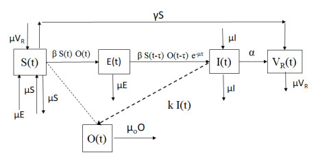
We propose a new mathematical model to investigate the effect of the introduction of an exposed stage for the cats who become infected with the T. gondii parasite, but that are not still able to produce oocysts in the environment. The model considers a time delay in order to represent the duration of the exposed stage. Besides the cat population the model also includes the oocysts related to the T. gondii in the environment. The model includes the cats since they are the only definitive host and the oocysts, since they are relevant to the dynamics of toxoplasmosis. The model considers lifelong immunity for the recovered cats and vaccinated cats. In addition, the model considers that cats can get infected through an effective contact with the oocysts in the environment. We find conditions such that the toxoplasmosis disease becomes extinct. We analyze the consequences of considering the exposed stage and the time delay on the stability of the equilibrium points. We numerically solve the constructed model and corroborated the theoretical results.

| [1] | CDC, Center for disease control and prevention, toxoplasmosis, 2021. Available from: https://www.cdc.gov/parasites/toxoplasmosis |
| [2] |
J. P. Dubey, Outbreaks of clinical toxoplasmosis in humans: Five decades of personal experience, perspectives and lessons learned, Parasite. Vector., 14 (2021), 1–12. https://doi.org/10.1186/s13071-021-04769-4 doi: 10.1186/s13071-021-04769-4

|
| [3] |
J. P. Dubey, The history of Toxoplasma gondii?the first 100 years, J. Eukaryot. Microbiol., 55 (2008), 467–475. https://doi.org/10.1111/j.1550-7408.2008.00345.x doi: 10.1111/j.1550-7408.2008.00345.x
|
| [4] |
M. Attias, D. E. Teixeira, M. Benchimol, R. C. Vommaro, P. H. Crepaldi, W. De Souza, The life-cycle of toxoplasma gondii reviewed using animations, Parasit. Vector., 13 (2020), 1–13. https://doi.org/10.1186/s13071-020-04445-z doi: 10.1186/s13071-020-04445-z
|
| [5] |
J. Dubey, History of the discovery of the life cycle of toxoplasma gondii, Int. J. Parasitol., 39 (2009), 877–882. https://doi.org/10.1016/j.ijpara.2009.01.005 doi: 10.1016/j.ijpara.2009.01.005
|
| [6] |
B. M. Di Genova, S. K. Wilson, J. Dubey, L. J. Knoll, Intestinal delta-6-desaturase activity determines host range for toxoplasma sexual reproduction, PLoS Biol., 17 (2019), e3000364. https://doi.org/10.1371/journal.pbio.3000364 doi: 10.1371/journal.pbio.3000364
|
| [7] |
J. Dubey, Advances in the life cycle of toxoplasma gondii, Int. J. Parasitol., 28 (1998), 1019–1024. https://doi.org/10.1016/S0020-7519(98)00023-X doi: 10.1016/S0020-7519(98)00023-X
|
| [8] |
F. Thomas, K. D. Lafferty, J. Brodeur, E. Elguero, M. Gauthier-Clerc, D. Missé, Incidence of adult brain cancers is higher in countries where the protozoan parasite toxoplasma gondii is common, Biol. Letters, 8 (2012), 101–103. https://doi.org/10.1098/rsbl.2011.0588 doi: 10.1098/rsbl.2011.0588
|
| [9] | J. Dubey, C. Beattie, Toxoplasmosis of Animals and Man, CRC Press, Boca Raton, FL., 1988. |
| [10] |
J. Dubey, D. Lindsay, C. Speer, Structures of Toxoplasma gondii tachyzoites, bradyzoites, and sporozoites and biology and development of tissue cysts, Clin. Microbiol. Rev., 11 (1998), 267–299. https://doi.org/10.1128/CMR.11.2.267 doi: 10.1128/CMR.11.2.267
|
| [11] |
J. Dubey, Duration of Immunity to Shedding of Toxoplasma gondii Oocysts by Cats, J. Parasitol., 81 (1995), 410–415. https://doi.org/10.2307/3283823 doi: 10.2307/3283823
|
| [12] |
J. A. Simon, R. Pradel, D. Aubert, R. Geers, I. Villena, M.-L. Poulle, A multi-event capture-recapture analysis of Toxoplasma gondii seroconversion dynamics in farm cats, Parasit. Vector., 11 (2018), 1–13. https://doi.org/10.1186/s13071-018-2834-4 doi: 10.1186/s13071-018-2834-4
|
| [13] |
J. Aramini, C. Stephen, J. P. Dubey, C. Engelstoft, H. Schwantje, C. S. Ribble, Potential contamination of drinking water with Toxoplasma gondii oocysts, Epidemiol. Infect., 122 (1999), 305–315. https://doi.org/10.1017/S0950268899002113 doi: 10.1017/S0950268899002113
|
| [14] |
J. P. Dubey, D. W. Thayer, C. A. Speer, S. K. Shen, Effect of gamma irradiation on unsporulated and sporulated Toxoplasma gondii oocysts, Int. J. Parasitol., 28 (1998), 369–375. https://doi.org/10.1016/S0020-7519(97)83432-7 doi: 10.1016/S0020-7519(97)83432-7
|
| [15] |
M. Lélu, M. Langlais, M.-L. Poulle, E. Gilot-Fromont, Transmission dynamics of Toxoplasma gondii along an urban–rural gradient, Theor. Popul. Biol., 78 (2010), 139–147. https://doi.org/10.1016/j.tpb.2010.05.005 doi: 10.1016/j.tpb.2010.05.005
|
| [16] |
A. A. B. Marinović, M. Opsteegh, H. Deng, A. W. Suijkerbuijk, P. F. van Gils, J. Van Der Giessen, Prospects of toxoplasmosis control by cat vaccination, Epidemics, 30 (2020), 100380. https://doi.org/10.1016/j.epidem.2019.100380 doi: 10.1016/j.epidem.2019.100380
|
| [17] | D. Trejos, I. Duarte, A mathematical model of dissemination of Toxoplasma gondii by cats, Actual. Biol., 27 (2005), 143–149. |
| [18] |
M. Turner, S. Lenhart, B. Rosenthal, X. Zhao, Modeling effective transmission pathways and control of the world?s most successful parasite, Theor. Popul. Biol., 86 (2013), 50–61. https://doi.org/10.1016/j.tpb.2013.04.001 doi: 10.1016/j.tpb.2013.04.001
|
| [19] |
H. Deng, R. Cummins, G. Schares, C. Trevisan, H. Enemark, H. Waap, et al., Mathematical modelling of Toxoplasma gondii transmission: A systematic review, Food Waterborne Parasitol., 22 (2021), e00102. https://doi.org/10.1016/j.fawpar.2020.e00102 doi: 10.1016/j.fawpar.2020.e00102
|
| [20] |
M. Lappin, Feline toxoplasmosis, In Pract., 21 (1999), 578–589. https://doi.org/10.1136/inpract.21.10.578 doi: 10.1136/inpract.21.10.578
|
| [21] | M. Sunquist, F. Sunquist, Wild Cats of the World, University of Chicago Press, 2002. |
| [22] |
D. Hill, J. Dubey, Toxoplasma gondii: Transmission, diagnosis and prevention, Clin. Microbiol. Infect., 8 (2002), 634–640. https://doi.org/10.1046/j.1469-0691.2002.00485.x doi: 10.1046/j.1469-0691.2002.00485.x
|
| [23] | B. Grenfell, A. Dobson, Ecology of Infectious Diseases in Natural Populations, Cambridge University Press, London, 1995. |
| [24] | F. Brauer, C. Castillo-Chavez, Mathematical models in population biology and epidemiology, Springer-Verlag, 2001. https://doi.org/10.1007/978-1-4614-1686-9 |
| [25] |
H. Hethcote, Mathematics of infectious diseases, SIAM Rev., 42 (2005), 599–653. https://doi.org/10.1137/S0036144500371907 doi: 10.1137/S0036144500371907
|
| [26] | J. D. Murray, Mathematical Biology I. An Introduction, Springer, Berlin, 2002. |
| [27] |
B. F. Kafsacka, V. B. Carruthers, F. J. Pineda, Kinetic modeling of toxoplasma gondii invasion, J. Theor. Biol., 249 (2007), 817–825. https://doi.org/10.1016/j.jtbi.2007.09.008 doi: 10.1016/j.jtbi.2007.09.008
|
| [28] |
G. C. González-Parra, A. J. Arenas, D. F. Aranda, R. J. Villanueva, L. Jódar, Dynamics of a model of toxoplasmosis disease in human and cat populations, Computers Math. Appl., 57 (2009), 1692–1700. https://doi.org/10.1016/j.camwa.2008.09.012 doi: 10.1016/j.camwa.2008.09.012
|
| [29] |
A. Sullivan, F. Agusto, S. Bewick, C. Su, S. Lenhart, X. Zhao, A mathematical model for within-host toxoplasma gondii invasion dynamics, Math. Biosci. Eng., 9 (2012), 647. https://doi.org/10.3934/mbe.2012.9.647 doi: 10.3934/mbe.2012.9.647
|
| [30] |
O. M. Ogunmiloro, Mathematical modeling of the coinfection dynamics of malaria-toxoplasmosis in the tropics, Biometr. Letters, 56 (2019), 139–163. https://doi.org/10.2478/bile-2019-0013 doi: 10.2478/bile-2019-0013
|
| [31] |
B. M. Chen-Charpentier, M. Jackson, Direct and indirect optimal control applied to plant virus propagation with seasonality and delays, J. Comput. Appl. Math., 380 (2020), 112983. https://doi.org/10.1016/j.cam.2020.112983 doi: 10.1016/j.cam.2020.112983
|
| [32] | Y. Kuang, Delay differential equations, University of California Press, 2012. |
| [33] | H. L. Smith, An introduction to delay differential equations with applications to the life sciences, vol. 57, Springer-Verlag New York, 2011. https://doi.org/10.1007/978-1-4419-7646-8 |
| [34] | F. A. Rihan, Delay differential equations and applications to biology, Springer, 2021. https://doi.org/10.1007/978-981-16-0626-7 |
| [35] |
H. Hethcote, P. Driessche, An SIS epidemic model with variable population size and a delay, J. Math. Biol., 34 (1995), 177–194. https://doi.org/10.1007/BF00178772 doi: 10.1007/BF00178772
|
| [36] |
P. Yan, S. Liu, SEIR epidemic model with delay, ANZIAM J., 48 (2006), 119–134. https://doi.org/10.1017/S144618110000345X doi: 10.1017/S144618110000345X
|
| [37] |
P. W. Nelson, J. D. Murray, A. S. Perelson, A model of HIV-1 pathogenesis that includes an intracellular delay, Math. Biosci., 163 (2000), 201–215. https://doi.org/10.1016/S0025-5564(99)00055-3 doi: 10.1016/S0025-5564(99)00055-3
|
| [38] |
O. Ogunmiloro, A. Idowu, On the existence of invariant domain and local asymptotic behavior of a delayed onchocerciasis model, Int. J. Modern Phys. C, 31 (2020), 2050142. https://doi.org/10.1142/S0129183120501429 doi: 10.1142/S0129183120501429
|
| [39] |
J. Li, G.-Q. Sun, Z. Jin, Pattern formation of an epidemic model with time delay, Phys. A Stat. Mechan. Appl., 403 (2014), 100–109. https://doi.org/10.1016/j.physa.2014.02.025 doi: 10.1016/j.physa.2014.02.025
|
| [40] | O. Arino, M. L. Hbid, E. A. Dads, Delay Differential Equations and Applications: Proceedings of the NATO Advanced Study Institute held in Marrakech, Morocco, 9-21 September 2002, vol. 205, Springer Science & Business Media, 2007. https://doi.org/10.1007/1-4020-3647-7 |
| [41] |
B.-Z. Guo, L.-M. Cai, A note for the global stability of a delay differential equation of hepatitis B virus infection, Math. Biosci. Eng., 8 (2011), 689–694. https://doi.org/10.3934/mbe.2011.8.689 doi: 10.3934/mbe.2011.8.689
|
| [42] |
M. Jackson, B. M. Chen-Charpentier, A model of biological control of plant virus propagation with delays, J. Comput. Appl. Math., 330 (2018), 855–865. https://doi.org/10.1016/j.cam.2017.01.005 doi: 10.1016/j.cam.2017.01.005
|
| [43] |
G. P. Samanta, Dynamic behaviour for a nonautonomous heroin epidemic model with time delay, J. Appl. Math. Comput., 35 (2011), 161–178. https://doi.org/10.1007/s12190-009-0349-z doi: 10.1007/s12190-009-0349-z
|
| [44] |
R. Xu, Global dynamics of an {SEIS} epidemiological model with time delay describing a latent period, Math. Computers Simul., 85 (2012), 90–102. https://doi.org/10.1016/j.matcom.2012.10.004 doi: 10.1016/j.matcom.2012.10.004
|
| [45] |
M. Bachar, On periodic solutions of delay differential equations with impulses, Symmetry, 11 (2019), 523. https://doi.org/10.3390/sym11040523 doi: 10.3390/sym11040523
|
| [46] | S. Busenberg, K. Cooke, Vertically transmitted diseases: Models and dynamics, vol. 23, Springer Science & Business Media, 2012. https://doi.org/10.1007/978-3-642-75301-5 |
| [47] | D. Breda, S. Maset, R. Vermiglio, Stability of linear delay differential equations: A numerical approach with MATLAB, Springer, 2014. https://doi.org/10.1007/978-1-4939-2107-2 |
| [48] |
J.-H. He, Periodic solutions and bifurcations of delay-differential equations, Phys. Letters A, 347 (2005), 228–230. https://doi.org/10.1016/j.physleta.2005.08.014 doi: 10.1016/j.physleta.2005.08.014
|
| [49] |
M. Á. Castro, M. A. García, J. A. Martín, F. Rodríguez, Exact and nonstandard finite difference schemes for coupled linear delay differential systems, Mathematics, 7 (2019), 1038. https://doi.org/10.3390/math7111038 doi: 10.3390/math7111038
|
| [50] |
A. El-Ajou, N. O. Moa'ath, Z. Al-Zhour, S. Momani, Analytical numerical solutions of the fractional multi-pantograph system: Two attractive methods and comparisons, Results Phys., 14 (2019), 102500. https://doi.org/10.1016/j.rinp.2019.102500 doi: 10.1016/j.rinp.2019.102500
|
| [51] |
M. García, M. Castro, J. A. Martín, F. Rodríguez, Exact and nonstandard numerical schemes for linear delay differential models, Appl. Math. Comput., 338 (2018), 337–345. https://doi.org/10.1016/j.amc.2018.06.029 doi: 10.1016/j.amc.2018.06.029
|
| [52] |
L. F. Shampine, S. Thompson, Solving ddes in matlab, Appl. Numer. Math.s, 37 (2001), 441–458. https://doi.org/10.1016/S0168-9274(00)00055-6 doi: 10.1016/S0168-9274(00)00055-6
|
| [53] |
G. Kerr, G. González-Parra, Accuracy of the Laplace transform method for linear neutral delay differential equations, Math. Computers Simul., 197 (2022), 308–326. https://doi.org/10.1016/j.matcom.2022.02.017 doi: 10.1016/j.matcom.2022.02.017
|
| [54] |
G. Kerr, G. González-Parra, M. Sherman, A new method based on the Laplace transform and Fourier series for solving linear neutral delay differential equations, Appl. Math. Comput., 420 (2022), 126914. https://doi.org/10.1016/j.amc.2021.126914 doi: 10.1016/j.amc.2021.126914
|
| [55] | L. F. Shampine, S. Thompson, Numerical solution of delay differential equations, in Delay Differential Equations, Springer, 2009, 1–27. https://doi.org/10.1007/978-0-387-85595-0 |
| [56] |
D. R. Willé, C. T. Baker, DELSOL-a numerical code for the solution of systems of delay-differential equations, Appl. Numer. Math., 9 (1992), 223–234. https://doi.org/10.1016/0168-9274(92)90017-8 doi: 10.1016/0168-9274(92)90017-8
|
| [57] |
J. Frenkel, J. Dubey, N. L. Miller, Toxoplasma gondii in cats: Fecal stages identified as coccidian oocysts, Science, 167 (1970), 893–896. https://doi.org/10.1126/science.167.3919.893 doi: 10.1126/science.167.3919.893
|
| [58] |
J. Frenkel, A. Ruiz, M. Chinchilla, Soil survival of Toxoplasma oocysts in Kansas and Costa Rica, Am. J. Trop. Med. Hyg., 24 (1975), 439–443. https://doi.org/10.4269/ajtmh.1975.24.439 doi: 10.4269/ajtmh.1975.24.439
|
| [59] |
L. Sibley, J. Boothroyd, Virulent strains of Toxoplasma gondii comprise a single clonal lineage, Nature, 359 (1992), 82–85. https://doi.org/10.1038/359082a0 doi: 10.1038/359082a0
|
| [60] |
A. J. Arenas, G. González-Parra, R.-J. V. Micó, Modeling toxoplasmosis spread in cat populations under vaccination, Theor. Popul. Biol., 77 (2010), 227–237. https://doi.org/10.1016/j.tpb.2010.03.005 doi: 10.1016/j.tpb.2010.03.005
|
| [61] |
G. González-Parra, S. Sultana, A. J. Arenas, Mathematical modeling of toxoplasmosis considering a time delay in the infectivity of oocysts, Mathematics, 10 (2022), 354. https://doi.org/10.3390/math10030354 doi: 10.3390/math10030354
|
| [62] |
J. Dubey, D. S. Lindsay, M. R. Lappin, Toxoplasmosis and other intestinal coccidial infections in cats and dogs, Vet. Clin. Small Animal Pract., 39 (2009), 1009–1034. https://doi.org/10.1016/j.cvsm.2009.08.001 doi: 10.1016/j.cvsm.2009.08.001
|
| [63] |
W. Jiang, A. M. Sullivan, C. Su, X. Zhao, An agent-based model for the transmission dynamics of toxoplasma gondii, J. Theor. Biol., 293 (2012), 15–26. https://doi.org/10.1016/j.jtbi.2011.10.006 doi: 10.1016/j.jtbi.2011.10.006
|
| [64] |
P. van den Driessche, J. Watmough, Reproduction numbers and sub-threshold endemic equilibria for compartmental models of disease transmission, Math. Biosci., 180 (2002), 29–48. https://doi.org/10.1016/S0025-5564(02)00108-6 doi: 10.1016/S0025-5564(02)00108-6
|
| [65] | P. van den Driessche, J. Watmough, Further notes on the basic reproduction number, in Math. Epidemiol., Springer, 2008,159–178. https://doi.org/10.1007/978-3-540-78911-6 |
| [66] |
E. A. Innes, C. Hamilton, J. L. Garcia, A. Chryssafidis, D. Smith, A one health approach to vaccines against Toxoplasma gondii, Food Waterborne Parasitol., 15 (2019), e00053. https://doi.org/10.1016/j.fawpar.2019.e00053 doi: 10.1016/j.fawpar.2019.e00053
|
| [67] |
D. Sykes, J. Rychtář, A game-theoretic approach to valuating toxoplasmosis vaccination strategies, Theor. Popul. Biol., 105 (2015), 33–38. https://doi.org/10.1016/j.tpb.2015.08.003 doi: 10.1016/j.tpb.2015.08.003
|
| [68] |
N. Mateus-Pinilla, B. Hannon, R. Weigel, A computer simulation of the prevention of the transmission of Toxoplasma gondii on swine farms using a feline T. gondii vaccine, Prevent. Vet. Med., 55 (2002), 17–36. https://doi.org/10.1016/S0167-5877(02)00057-0 doi: 10.1016/S0167-5877(02)00057-0
|
| [69] |
A. Freyre, L. Choromanski, J. Fishback, I. Popiel, Immunization of cats with tissue cysts, bradyzoites, and tachyzoites of the T-263 strain of Toxoplasma gondii, J. Parasitol., 79 (1993), 716–719. https://doi.org/10.2307/3283610 doi: 10.2307/3283610
|
| [70] | J. Frenkel, Transmission of toxoplasmosis and the role of immunity in limiting transmission and illness, J. Am. Vet. Med. Assoc., 196 (1990), 233–240. |
| [71] |
M. R. Islam, T. Oraby, A. McCombs, M. M. Chowdhury, M. Al-Mamun, M. G. Tyshenko, et al., Evaluation of the United States COVID-19 vaccine allocation strategy, PloS One, 16 (2021), e0259700. https://doi.org/10.1371/journal.pone.0259700 doi: 10.1371/journal.pone.0259700
|
| [72] |
G. González-Parra, M. R. Cogollo, A. J. Arenas, Mathematical modeling to study optimal allocation of vaccines against covid-19 using an age-structured population, Axioms, 11 (2022), 109. https://doi.org/10.3390/axioms11030109 doi: 10.3390/axioms11030109
|
| [73] |
J. Dubey, M. Mattix, T. Lipscomb, Lesions of neonatally induced toxoplasmosis in cats, Vet. Pathol., 33 (1996), 290–295. https://doi.org/10.1177/030098589603300305 doi: 10.1177/030098589603300305
|
| [74] |
C. C. Powell, M. R. Lappin, Clinical ocular toxoplasmosis in neonatal kittens, Vet. Ophthalmol., 4 (2001), 87–92. https://doi.org/10.1046/j.1463-5224.2001.00180.x doi: 10.1046/j.1463-5224.2001.00180.x
|
| [75] |
K. Sato, I. Iwamoto, K. Yoshiki, Experimental toxoplasmosis in pregnant cats, Vet. Ophthalmol., 55 (1993), 1005–1009. https://doi.org/10.1292/jvms.55.1005 doi: 10.1292/jvms.55.1005
|
| [76] | J. Dubey, M. Lappin and P. Thulliez, Diagnosis of induced toxoplasmosis in neonatal cats, J. Am. Vet. Med. Assoc., 207 (1995), 179–185. |
| [77] |
C. C. Powell, M. Brewer, M. R. Lappin, Detection of toxoplasma gondii in the milk of experimentally infected lactating cats, Vet. Parasitol., 102 (2001), 29–33. https://doi.org/10.1016/S0304-4017(01)00521-0 doi: 10.1016/S0304-4017(01)00521-0
|
| [78] | V. Lakshmikantham, S. Leela, A. Martynyuk, Stability Analysis of Nonlinear Systems, Marcel Dekker, Inc., New York and Basel, 1989. https://doi.org/10.1007/978-3-319-27200-9 |
| [79] | J. P. La Salle, The stability of dynamical systems, SIAM, 1976. |
| [80] |
K. Berthier, M. Langlais, P. Auger, D. Pontier, Dynamics of a feline virus with two transmission modes within exponentially growing host populations, Proceed. Royal Soc. B Biol. Sci., 267 (2000), 2049–2056. https://doi.org/10.1098/rspb.2000.1248 doi: 10.1098/rspb.2000.1248
|
| [81] | R. Fayer, Toxoplasmosis update and public health implications, Canadian Vet. J., 22 (1981), 344. |
| [82] |
A. L. Lloyd, Realistic distributions of infectious periods in epidemic models: changing patterns of persistence and dynamics, Theoret. Popul. Biol., 60 (2001), 59–71. https://doi.org/10.1006/tpbi.2001.1525 doi: 10.1006/tpbi.2001.1525
|
| [83] |
G. González-Parra, F. De Ridder, D. Huntjens, D. Roymans, G. Ispas, H. M. Dobrovolny, A comparison of RSV and influenza in vitro kinetic parameters reveals differences in infecting time, PloS one, 13 (2018), e0192645. https://doi.org/10.1371/journal.pone.0192645 doi: 10.1371/journal.pone.0192645
|
| [84] |
G. González-Parra, H. M. Dobrovolny, D. F. Aranda, B. Chen-Charpentier, R. A. G. Rojas, Quantifying rotavirus kinetics in the REH tumor cell line using in vitro data, Virus Res., 244 (2018), 53–63. https://doi.org/10.1016/j.virusres.2017.09.023 doi: 10.1016/j.virusres.2017.09.023
|
| [85] |
X. Wang, Y. Shi, Z. Feng, J. Cui, Evaluations of interventions using mathematical models with exponential and non-exponential distributions for disease stages: The case of Ebola, Bullet. Math. Biol., 79 (2017), 2149–2173. https://doi.org/10.1007/s11538-017-0324-z doi: 10.1007/s11538-017-0324-z
|


Figures(6) / Tables(1)

Sharmin Sultana, Gilberto González-Parra, Abraham J. Arenas. Dynamics of toxoplasmosis in the cat's population with an exposed stage and a time delay[J]. Mathematical Biosciences and Engineering, 2022, 19(12): 12655-12676. doi: 10.3934/mbe.2022591


 DownLoad: