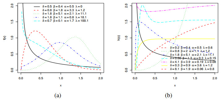
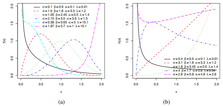
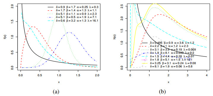
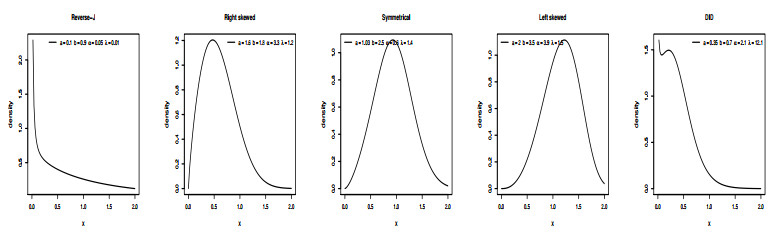
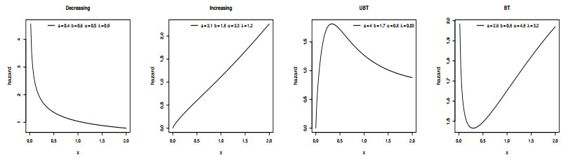
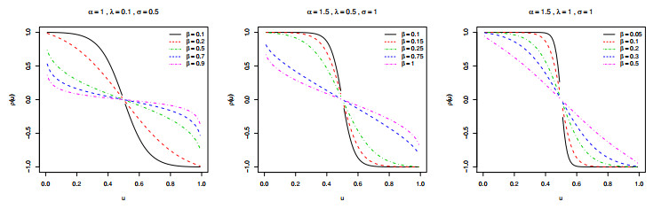
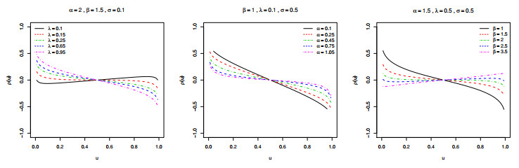
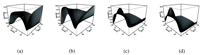
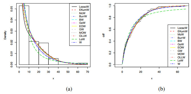
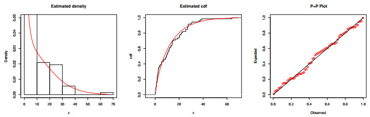
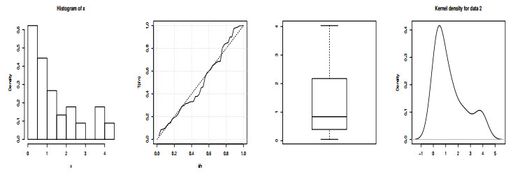
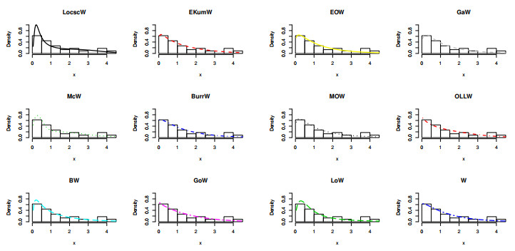
The modern trend in distribution theory is to propose hybrid generators and generalized families using existing algebraic generators along with some trigonometric functions to offer unique, more flexible, more efficient, and highly productive G-distributions to deal with new data sets emerging in different fields of applied research. This article aims to originate an odd sine generator of distributions and construct a new G-family called "The Odd Lomax Trigonometric Generalized Family of Distributions". The new densities, useful functions, and significant characteristics are thoroughly determined. Several specific models are also presented, along with graphical analysis and detailed description. A new distribution, "The Lomax cosecant Weibull" (LocscW), is studied in detail. The versatility, robustness, and competency of the LocscW model are confirmed by applications on hydrological and survival data sets. The skewness and kurtosis present in this model are explained using modern graphical methods, while the estimation and statistical inference are explored using many estimation approaches.
Citation: M. E. Bakr, Abdulhakim A. Al-Babtain, Zafar Mahmood, R. A. Aldallal, Saima Khan Khosa, M. M. Abd El-Raouf, Eslam Hussam, Ahmed M. Gemeay. Statistical modelling for a new family of generalized distributions with real data applications[J]. Mathematical Biosciences and Engineering, 2022, 19(9): 8705-8740. doi: 10.3934/mbe.2022404
The modern trend in distribution theory is to propose hybrid generators and generalized families using existing algebraic generators along with some trigonometric functions to offer unique, more flexible, more efficient, and highly productive G-distributions to deal with new data sets emerging in different fields of applied research. This article aims to originate an odd sine generator of distributions and construct a new G-family called "The Odd Lomax Trigonometric Generalized Family of Distributions". The new densities, useful functions, and significant characteristics are thoroughly determined. Several specific models are also presented, along with graphical analysis and detailed description. A new distribution, "The Lomax cosecant Weibull" (LocscW), is studied in detail. The versatility, robustness, and competency of the LocscW model are confirmed by applications on hydrological and survival data sets. The skewness and kurtosis present in this model are explained using modern graphical methods, while the estimation and statistical inference are explored using many estimation approaches.

| [1] |
C. Lee, F. Famoye, A. Y. Alzaatreh, Methods for generating families of univariate continuous distributions in the recent decades, WIREs Comput. Stat., 5 (2013), 219–238. https://doi.org/10.1002/wics.1255 doi: 10.1002/wics.1255

|
| [2] | A. A. Al-Babtain, I. Elbatal, H. Al-Mofleh, A. M. Gemeay, A. Z. Afify, A. M. Sarg, The flexible burr XG family: properties, inference, and applications in engineering science symmetry, 13 (2021), 474. https://doi.org/10.3390/sym13030474 |
| [3] |
A. E. A. Teamah, A. A. Elbanna, A. M. Gemeay, Right truncated fréchet-weibull distribution: statistical properties and application, Delta J. Sci., 41 (2020), 20–29. https://doi.org/10.21608/djs.2020.139880 doi: 10.21608/djs.2020.139880
|
| [4] |
A. E. A. Teamah, A. A. Elbanna, A. M. Gemeay, Heavy-tailed log-logistic distribution: properties, risk measures and applications, Stat., Optim. Inf. Comput., 9 (2021), 910–941. https://doi.org/10.19139/soic-2310-5070-1220 doi: 10.19139/soic-2310-5070-1220
|
| [5] |
M. H. Tahir, S. Nadarajah, Parameter induction in continuous univariate distributions: Well-established G families, Ann. Acad. Bras. Cienc., 87 (2015), 539–568. https://doi.org/10.1590/0001-3765201520140299 doi: 10.1590/0001-3765201520140299
|
| [6] |
S. Shamshirband, M. Fathi, A. Dehzangi, A. T. Chronopoulos, H. Alinejad-Rokny, A review on deep learning approaches in healthcare systems: Taxonomies, challenges, and open issues, J. Biomed. Inf., 113 (2021), 103627. https://doi.org/10.1016/j.jbi.2020.103627 doi: 10.1016/j.jbi.2020.103627
|
| [7] |
S. Shamshirband, J. H. Joloudari, S. K. Shirkharkolaie, S. Mojrian, F. Rahmani, S. Mostafavi, et al., Game theory and evolutionary optimization approaches applied to resource allocation problems in computing environments: A survey, Math. Biosci. Eng., 18 (2021), 9190–9232. https://doi.org/10.3934/mbe.2021453 doi: 10.3934/mbe.2021453
|
| [8] |
J. H. Joloudari, E. H. Joloudari, H. Saadatfar, M. Ghasemigol, S. M. Razavi, A. Mosavi, et al., Coronary artery disease diagnosis; ranking the significant features using a random trees model, Int. J. Environ. Res. Public Health, 17 (2020), 731. https://doi.org/10.3390/ijerph17030731 doi: 10.3390/ijerph17030731
|
| [9] | J. U. Gleaton, J. D. Lynch, Properties of generalized log-logistic families of lifetime distributions, J. Probab. Stat., 4 (2006), 51–64. |
| [10] | M. Bourguignon, R. B. Silva, G. M. Cordeiro, The Weibull–G family of probability distributions, J. Data Sci., 12 (2014), 53–68. Available from: https://www.jds-online.com/files/JDS-1210.pdf. |
| [11] | D. Kumar, U. Singh, S. K. Singh, A new distribution using sine function- Its application to bladder cancer patients data, J. Stat. Appl. Probab. Lett., 4 (2015), 417–427. Available from: https://www.naturalspublishing.com/files/published/j9wsil53h390x8.pdf. |
| [12] |
B. Hosseini, M. Afshari, M. Alizadeh, The generalized odd Gamma-G family of distributions: properties and applications, Austrian J. Stat., 47 (2018), 69–89. https://doi.org/10.17713/ajs.v47i2.580 doi: 10.17713/ajs.v47i2.580
|
| [13] | J. F. Kenney, E. S. Keeping, Mathematics of Statistics, Chapman and Hall Ltd, New Jersey, 1962. |
| [14] |
J. J. Moors, A quantile alternative for kurtosis, J. R. Stat. Soc., Ser. D, 37 (1988), 25–32. https://doi.org/10.2307/2348376 doi: 10.2307/2348376
|
| [15] |
E. Parzen, Nonparametric statistical modelling, J. Am. Stat. Assoc., 74 (1979), 105–121. https://doi.org/10.1080/01621459.1979.10481621 doi: 10.1080/01621459.1979.10481621
|
| [16] | M. Shaked, J. G. Shanthikumar, Stochastic Orders and Their Applications, Academic Press, New York, 1994. |
| [17] | S. Kotz, Y. Lumelskii, M. Penskey, The Stress-strength Model and Its Generalizations: Theory and Applications, World Scientific, Singapore, 2003. |
| [18] | H. A. David, H. N. Nagaraja, Order Statistics, John Wiley and Sons, New Jersey, 2003. |
| [19] |
F. H. Riad, E. Hussam, A. M. Gemeay, R. A. Aldallal, A. Z. Afify, Classical and Bayesian inference of the weighted-exponential distribution with an application to insurance data, Math. Biosci. Eng., 19 (2022), 6551–6581. https://doi.org/10.3934/mbe.2022309 doi: 10.3934/mbe.2022309
|
| [20] |
H. M. Alshanbari, A. M. Gemeay, A. A. A. H. El-Bagoury, S. K. Khosa, E. H. Hafez, A. H. Muse, A novel extension of Fréchet distribution: Application on real data and simulation, Alexandria Eng. J., 61 (2022), 7917–7938. https://doi.org/10.1016/j.aej.2022.01.013 doi: 10.1016/j.aej.2022.01.013
|
| [21] |
A. Z. Afify, H. M. Aljohani, A. S. Alghamdi, A. M. Gemeay, A. M. Sarg, A new two-parameter Burr-Hatke distribution: properties and bayesian and non-bayesian inference with applications, J. Math., 2021. https://doi.org/10.1155/2021/1061083 doi: 10.1155/2021/1061083
|
Figures(19) / Tables(13)

M. E. Bakr, Abdulhakim A. Al-Babtain, Zafar Mahmood, R. A. Aldallal, Saima Khan Khosa, M. M. Abd El-Raouf, Eslam Hussam, Ahmed M. Gemeay. Statistical modelling for a new family of generalized distributions with real data applications[J]. Mathematical Biosciences and Engineering, 2022, 19(9): 8705-8740. doi: 10.3934/mbe.2022404


 DownLoad: