
The redesign of national curricula across the Anglophone world since the 1990s is demonstrably shaped by common policy trends. Focusing on the profound and uncritiqued changes that have been implemented in New Zealand education, this paper provides a critical commentary on the characterising features of the current New Zealand mathematics curriculum, describing a context within which mathematics education at schools is severely compromised. Drawing on the evidence available from large-scale international indicators, such as PISA and TIMSS, to benchmark associated curriculum changes implemented by the New Zealand government, we hypothesise that the ongoing decline of student mathematical achievement is the result of four main interdependent features which characterise the New Zealand curriculum. The features are (1) its highly generic non-prescriptive nature, (2) a commitment to teacher autonomy in curriculum knowledge selection, (3) competency-based outcomes approach, and (4) a commitment to localisation in curriculum selection. Recognising socio-political forces and ideological and intellectual ideas associated with those forces, we discuss each characterising feature, in turn, to show how they contribute to and draw from the others to create a 'curriculum without content'. We conclude with explicit recommendations and a call for future studies to establish the extent to which each of these four features contributes to the decline of student achievement.
Citation: Neil Morrow, Elizabeth Rata, Tanya Evans. The New Zealand mathematics curriculum: A critical commentary[J]. STEM Education, 2022, 2(1): 59-72. doi: 10.3934/steme.2022004
[1] | Ihtisham Ul Haq, Shabir Ahmad, Sayed Saifullah, Kamsing Nonlaopon, Ali Akgül . Analysis of fractal fractional Lorenz type and financial chaotic systems with exponential decay kernels. AIMS Mathematics, 2022, 7(10): 18809-18823. doi: 10.3934/math.20221035 |
[2] | A. E. Matouk . Chaos and hidden chaos in a 4D dynamical system using the fractal-fractional operators. AIMS Mathematics, 2025, 10(3): 6233-6257. doi: 10.3934/math.2025284 |
[3] | Nehad Ali Shah, Iftikhar Ahmed, Kanayo K. Asogwa, Azhar Ali Zafar, Wajaree Weera, Ali Akgül . Numerical study of a nonlinear fractional chaotic Chua's circuit. AIMS Mathematics, 2023, 8(1): 1636-1655. doi: 10.3934/math.2023083 |
[4] | A. M. Alqahtani, Shivani Sharma, Arun Chaudhary, Aditya Sharma . Application of Caputo-Fabrizio derivative in circuit realization. AIMS Mathematics, 2025, 10(2): 2415-2443. doi: 10.3934/math.2025113 |
[5] | Shabir Ahmad, Aman Ullah, Mohammad Partohaghighi, Sayed Saifullah, Ali Akgül, Fahd Jarad . Oscillatory and complex behaviour of Caputo-Fabrizio fractional order HIV-1 infection model. AIMS Mathematics, 2022, 7(3): 4778-4792. doi: 10.3934/math.2022265 |
[6] | Rahat Zarin, Abdur Raouf, Amir Khan, Aeshah A. Raezah, Usa Wannasingha Humphries . Computational modeling of financial crime population dynamics under different fractional operators. AIMS Mathematics, 2023, 8(9): 20755-20789. doi: 10.3934/math.20231058 |
[7] | Khalid K. Ali, K. R. Raslan, Amira Abd-Elall Ibrahim, Mohamed S. Mohamed . On study the fractional Caputo-Fabrizio integro differential equation including the fractional q-integral of the Riemann-Liouville type. AIMS Mathematics, 2023, 8(8): 18206-18222. doi: 10.3934/math.2023925 |
[8] | Sarkhel Akbar Mahmood, Pshtiwan Othman Mohammed, Dumitru Baleanu, Hassen Aydi, Yasser S. Hamed . Analysing discrete fractional operators with exponential kernel for positivity in lower boundedness. AIMS Mathematics, 2022, 7(6): 10387-10399. doi: 10.3934/math.2022579 |
[9] | Xiaoyong Xu, Fengying Zhou . Orthonormal Euler wavelets method for time-fractional Cattaneo equation with Caputo-Fabrizio derivative. AIMS Mathematics, 2023, 8(2): 2736-2762. doi: 10.3934/math.2023144 |
[10] | Rahat Zarin, Amir Khan, Pushpendra Kumar, Usa Wannasingha Humphries . Fractional-order dynamics of Chagas-HIV epidemic model with different fractional operators. AIMS Mathematics, 2022, 7(10): 18897-18924. doi: 10.3934/math.20221041 |
The redesign of national curricula across the Anglophone world since the 1990s is demonstrably shaped by common policy trends. Focusing on the profound and uncritiqued changes that have been implemented in New Zealand education, this paper provides a critical commentary on the characterising features of the current New Zealand mathematics curriculum, describing a context within which mathematics education at schools is severely compromised. Drawing on the evidence available from large-scale international indicators, such as PISA and TIMSS, to benchmark associated curriculum changes implemented by the New Zealand government, we hypothesise that the ongoing decline of student mathematical achievement is the result of four main interdependent features which characterise the New Zealand curriculum. The features are (1) its highly generic non-prescriptive nature, (2) a commitment to teacher autonomy in curriculum knowledge selection, (3) competency-based outcomes approach, and (4) a commitment to localisation in curriculum selection. Recognising socio-political forces and ideological and intellectual ideas associated with those forces, we discuss each characterising feature, in turn, to show how they contribute to and draw from the others to create a 'curriculum without content'. We conclude with explicit recommendations and a call for future studies to establish the extent to which each of these four features contributes to the decline of student achievement.
The complexities of physical phenomena in nature have forced researchers into developing mathematical models that can be used to describe and capture the behavior of these natural occurrences. Traditional calculus may seem to be enough in solving problems that arise from science and engineering. However, many physical phenomena may better be described by fractional calculus because it is a well-suited tool to analyze problems of fractal dimension, with long term "memory" and chaotic behavior [1]. Some of the advantages of using fractional calculus over classical calculus are presented by authors in [2,3,4,5]. Even though fractional calculus was initially a pure mathematics idea and now regarded as a part of applied mathematics, its application has spread to other fields such as physics [3,6], economy [4], biology [3,5,7,8,9,10], probability[11], signal processing [12], quantitative biology, elasticity, diffusion process, systems identification, viscoelasticity [13], transport theory, electrochemistry, rheology, control theory, potential theory, and scattering theory [14,15]. Many authors have looked at the theoretical results based on the well-posedness of the fractional differential equations in different forms [16,17,18,19]. It is clear that for most fractional differential problems, analytical solutions are either impossible to find or are only possible under unrealistic simplifications. As a result, different numerical techniques have been presented by many authors, among which are the variational iteration method, finite difference schemes, Adomain's decomposition, Fourier spectral methods, homotopy analysis methods, A two-step Adams-Bashforth method [20], Haar wavelet numerical method [21], and many others that have been presented in [22].
Another concept that has raised interest in researchers is chaotic systems. Chaotic behavior can be seen in a variety of systems such as fluid dynamics [23], population growth, the dynamics of molecular vibration, ecology, electric circuits, the time evolution of the magnetic field of celestial bodies, weather, mechanical devices, and laser [24]. Some of the applications of fractional calculus on systems that exhibit chaotic behavior are presented in [25,26,27,28,29,30]. In this study, we will consider a three-dimensional nonlinear chaotic system called the Lorenz chaotic system [31,32,33] introduced by Lorenz [34]. This chaotic system opened doors to the development of many other three-dimensional nonlinear chaotic systems such as stretch-twist-fold flow [30,35], Chen system [36], Rossler system [37] and Lui system [38].
Recently a new concept of differential and integral operators called fractal-fractional differential and integral operators were introduced by Atangana [39], as the convolution of the generalized Mittag-Leffler law, exponential law, and power-law with fractal derivative. These operators consist of two orders, firstly the fractional-order q then the fractal dimension k. The purpose of the new operators is to attract nonlocal problems in nature that also display fractal behavior. The fractal-fractional derivatives find their applications in long-term relation description, macro, and micro-scaled phenomena, discontinuous differential problems, anomalous physical processes [40,41,42]. Many authors have looked and these operators and applied them to different fields. Authors such as Qureshi and Atangana [43] presented a paper where they used fractal-fractional differentiation to model and analyzed mathematically the dynamics of the transmission of diarrhea that occurred in Ghana between the year 2008 and 2018. A similar study was done by Srivastava, and Saad [44]. In their case, they used fractional fractal operators to model the ebola virus. The idea of modeling using fractal fractional derivative was also used by Atangana et al. [16] for fractional reaction-diffusion equations. Atangana and Qureshi [45] presented a paper where they used the fractional fractal operators to predict chaotic behavior of the Modified Lu Chen attractor, Modified Chua chaotic attractor, Lu Chen attractor, and Chen attractor.
The rest of this paper is arranged in the following way. Under Section 2, we briefly discuss some of the properties and definitions used in this study. The Lorenz Chaotic system under the fractal fractional Caputo Fabrizio derivative is presented in Section 3. In Section 4, we look at the well-posedness of the solution. The numerical scheme is derived in 5. The numerical simulation and graphical results are presented in Section 6. Numerical discussion and error estimate in Sections 7. Lastly, the conclusion is in found Section 8.
In this section, we will give a brief discussion of some important definitions and properties from fractal-fractional calculus that are useful for this paper.
The following definitions are discussed in detail in [39].
Definition 2.1. [39] Suppose that u(t) is a continuous function and fractal differentiable on an open interval (a,b) with order k then, a q order fractal-fractional derivative of the function u(t) in a Caputo sense with a power-law type kernel is given by:
Dq,ka,t(u(t))=1Γ(n−q)∫tadu(s)dsk(t−s)n−q−1ds, | (2.1) |
where 0<n−1<q,k≤n∈N and
du(s)dsk=limt→su(x)−u(s)tk−sk. |
A generalized version of the above equation is defined as follows:
Dq,k,θa,t(u(t))=1Γ(n−q)∫tadθu(s)dsk(t−s)n−q−1ds, | (2.2) |
and
dθu(s)dsk=limt→suθ(x)−uθ(s)tk−sk, |
where θ≤1.
Definition 2.2. [39] Suppose that u(t) is a continuous function and fractal differentiable on an open interval (a,b) with order k then, a q order fractal-fractional derivative of the function u(t) in a Caputo sense with an exponential decay type kernel is given by:
Dq,ka,t(u(t))=M(q)1−q∫tadu(s)dskexp[−q1−q(t−s)]ds, | (2.3) |
where 0<q,k≤n∈N and M(0)=M(1)=1.
A generalized version of the above equation is defined as follows:
Dq,k,θa,t(u(t))=M(q)1−q∫tadθu(s)dskexp[−q1−q(t−s)]ds, | (2.4) |
where 0<q,k,θ≤1.
Definition 2.3. [39] Suppose that u(t) is a continuous function and fractal differentiable on an open interval (a,b) with order k then, a q order fractal-fractional derivative of the function u(t) in a Caputo sense with the generalized Mittag-Leffler kernel is given by:
Dq,ka,t(u(t))=AB(q)1−q∫tadu(s)dskEq(−q1−q(t−s)q)ds, | (2.5) |
A generalized version of the above equation is defined as follows:
Dq,k,θa,t(u(t))=AB(q)1−q∫tadθu(s)dskEq(−q1−q(t−s)q)ds, | (2.6) |
where 0<α,β≤1 and AB(α)=1−α+αΓ(α).
Definition 2.4. [39] Suppose that u(t) is a continuous function and fractal differentiable on an open interval (a,b) with order k then, a q order fractal-fractional derivative of the function u(t) in a Caputo sense with exponential decay kernel is given by:
Dq,ka,t(u(t))=M(q)(1−q)ddsk∫tau(s)exp[−q1−q(t−s)2]ds, | (2.7) |
where 0<q,k≤n and M(0)=M(1)=1.
A generalized version of the above equation is defined as follows:
Dq,k,θa,t(u(t))=M(q)(1−q)dθdsk∫tau(s)exp[−q1−q(t−s)2]ds, | (2.8) |
where 0<q,k,θ≤1.
Definition 2.5. [39] Assuming that u(t) is a continuous function on (a,b), then a q order fractal-fractional integral of the function u(t) with power law type kernel is given by:
Jq,ka,t(u(t))=kΓ(q)∫ta(t−s)q−1sk−1u(s)ds. | (2.9) |
Definition 2.6. [39] Assuming that u(t) is a continuous function on (a,b), then a q order fractal-fractional integral of the function u(t) with an exponential decaying type kernel is given by:
Jq,ka,t(u(t))=qkM(q)∫tasq−1u(s)ds+k(1−q)tk−1u(t)M(q). | (2.10) |
Definition 2.7. [39] Assuming that u(t) is a continuous function on (a,b), then a q order fractal-fractional integral of the function u(t) with a generalized Mittag-Leffler type kernel is given by:
Jq,ka,t(u(x))=qkAB(q)∫task−1u(s)(t−s)q−1ds+k(1−q)tk−1u(t)AB(q). | (2.11) |
In this section, we introduce the Lorenz chaotic system under the definition of fractal fractional Caputo-Fabrizio derivative.
Consider the following three dimensional nonlinear chaotic system called the Lorenz chaotic system [24,46]
x′(t)=γ(y−x),y′(t)=ρx−y−xz,z′(t)=xy−δz, | (3.1) |
where x=x(t), y=y(t), and z=z(t) are the dynamical variable of the system and γ, ρ, and δ are the related real constants parameters. Using the definition of the fractal-fractional derivative under the Riemann-Liouville sense with exponential decay kernel for each classical derivative equations in (3.1), we obtain
RLDq,k0,tx(t)=Φ1(x,y,z,t),RLDq,k0,ty(t)=Φ2(x,y,z,t),RLDq,k0,tz(t)=Φ3(x,y,z,t), | (3.2) |
where Φ1(x,y,z,t)=γ(y−x), Φ2(x,y,z,t)=ρx−y−xz, and Φ3(x,y,z,t)=xy−δz. The above system of equations can be written as follows
RLDq,k0,tx(t)=M(q)1−qddtk∫t0exp(−q1−q(t−s))Φ1(x,y,z,s)ds,RLDq,k0,ty(t)=M(q)1−qddtk∫t0exp(−q1−q(t−s))Φ2(x,y,z,s)ds,RLDq,k0,tz(t)=M(q)1−qddtk∫t0exp(−q1−q(t−s))Φ3(x,y,z,s)ds. | (3.3) |
Since the fractional integral is differentiable. We can rewrite the Eq (3.3) as
RLDq,k0,tx(t)=M(q)1−qddt∫t0exp(−q1−q(t−s))Φ1(x,y,z,s)ds1ktk−1,RLDq,k0,ty(t)=M(q)1−qddt∫t0exp(−q1−q(t−s))Φ2(x,y,z,s)ds1ktk−1,RLDq,k0,tz(t)=M(q)1−qddt∫t0exp(−q1−q(t−s))Φ3(x,y,z,s)ds1ktk−1. | (3.4) |
Therefore, system (3.4) can be expressed as follows
RLDq,k0,tx(t)=ktk−1Φ1(x,y,z,t),RLDq,k0,ty(t)=ktk−1Φ2(x,y,z,t),RLDq,k0,tz(t)=ktk−1Φ3(x,y,z,t). | (3.5) |
We now replace the Riemann-Liouville derivative with the Caputo-Fabrizio derivative to make use of the integer-order initial conditions. Thus from system (3.5) we get
CFDq,k0,tx(t)=ktk−1Φ1(x,y,z,t),CFDq,k0,ty(t)=ktk−1Φ2(x,y,z,t),CFDq,k0,tz(t)=ktk−1Φ3(x,y,z,t). | (3.6) |
In this study, we will investigate the above system of equations.
In this section, we use the Pichard Lindelof method [46,47,48] to show the existence and uniqueness of the solution of the following nonlinear system of equations
CFDq,k0,tx(t)=ktk−1Φ1(x,y,z,t),CFDq,k0,ty(t)=ktk−1Φ2(x,y,z,t),CFDq,k0,tz(t)=ktk−1Φ3(x,y,z,t), | (4.1) |
subjected to the following initial conditions
x(0)=x0,y(0)=y0,z(0)=z0. |
To show the existence and uniqueness of the solution we define the following operators.
f1(t,x)=γ(y−x),f2(t,y)=ρx−y−xz,f3(t,z)=xy−δz, | (4.2) |
Now, let
Ca,b1=A1×B1,Ca,b2=A2×B2,Ca,b3=A3×B3, | (4.3) |
where
A1=A2=A3=[t0−a,t0+a],B1=[x0−b1,x0+b1],B2=[y0−b2,y0+b2],B3=[z0−b3,z0+b3], | (4.4) |
We now want to show that f1,f2 and f3 satisfy the Lipschipitz conditions with respect to x,y,z respectively. This means that for any two given functions ψ1,ψ2∈C(A1,B1,B2,B3) there exists a positive constant k such that
‖f(t,ψ1)−f(t,ψ2)‖≤k‖ψ1−ψ2‖. |
For f1 we have
‖f1(t,ψ1)−f1(t,ψ2)‖=‖(γy(t)−γψ1))−(γy(t)−γψ2)‖=‖−γψ1+γψ2‖=‖−γ(ψ1−ψ2)‖≤|γ|‖ψ1−ψ2‖. | (4.5) |
Hence, f1 is satisfies the Lipschipitz conditions. For f2 we have
‖f2(t,ψ1)−f2(t,ψ2)‖=‖(ρx(t)−ψ1−x(t)z(t))−(ρx(t)−ψ2−x(t)z(t))‖=‖−ψ1+ψ2‖=‖−(ψ1−ψ2)‖≤‖ψ1−ψ2‖. | (4.6) |
Thus, f2 is satisfies the Lipschipitz conditions. For f3 we have
‖f3(t,ψ1)−f3(t,ψ2)‖=‖(x(t)y(t)−δψ1)−(x(t)y(t)−δψ2))‖=‖−δψ1+δψ2‖=‖−δ(ψ1−ψ2)‖≤|δ|‖ψ1−ψ2‖. | (4.7) |
Therefore, f3 satisfies the Lipschipitz conditions.
Now, let
M1=supCa,b1|f1(t,x)|,M2=supCa,b2|f2(t,y)|,M3=supCa,b3|f3(t,z)|, | (4.8) |
We now continue to apply the Banach fixed point theorem using the metric on spaces of continuous functions C(A1,B1,B2,B3) induced by the norm
‖f(t)‖∞=supt∈[t0−a,t0+a]|f(t)|. | (4.9) |
We now define the next operator between the two functional spaces of continuous functions, Picard's operator, as follows
D:C(A1,B1,B2,B3)→C(A1,B1,B2,B3). | (4.10) |
Defined as follows
DX(t)=X0(t)+ktk−1(1−q)M(q)F(t,X(t))+qkM(q)∫t0Λτ−1F(Λ,X(Λ))dΛ | (4.11) |
Where the matrix X is given as
X(t)=[x(t)y(t)z(t)] |
X0(t)=[x0y0z0] |
and
F(t,X(t))=[f1(t,x)f2(t,y)f3(t,z)] |
From (4.5)–(4.7) we can conclude that F(t,X(t)) satisfies Lipschipitz conditions with respect to the system state variable X(t). Now, we must show that this operator maps a complete nonempty space into itself. We first show that, given a certain restriction on a, D takes values in B1,B2,B3 in the space of continuous functions with uniform norm. To obtain good results, we assume that the problem under consideration satisfies
‖X(t)‖∞=max{b1,b2,b3}=b |
implies
‖DX(t)−X0(t)‖=‖ktk−1(1−q)M(q)F(t,X(t))+qkM(q)∫t0Λk−1F(Λ,X(Λ))dΛ‖≤ktk−1(1−q)M(q)‖F(t,X(t))‖+qkM(q)∫t0Λk−1‖F(Λ,X(Λ))dΛ‖≤ktk−1(1−q)M(q)M+qkM(q).Makk≤Ma≤b, | (4.12) |
where b=max{b1,b2,b3} and M=max{M1,M2,M3}. The last step is true if we impose the requirement a<bM.
Using the maximum's metric
‖DX1−DX2‖∞=supt∈[t0−a,t0+a]|X1−X2|. | (4.13) |
We want to show that the operator is a contraction mapping. So, we have
‖DX(t)−X0(t)‖=‖tk−1(1−q)M(q)[F(t,X1(t))−F(t,X2(t))]+qkM(q)∫t0Λk−1[F(Λ,X1(Λ))−F(Λ,X2(Λ))]dΛ‖≤ktk−1(1−q)M(q)‖F(t,X1(t))−F(t,X2(t))‖+qkM(q)∫t0λk−1‖F(Λ,X1(Λ))−F(Λ,X2(Λ))‖dΛ≤ktk−1(1−q)M(q)p‖X1(t)−X2(t)‖+qkM(q)∫t0Λk−1‖F(Λ,X1(Λ))−F(Λ,X2(Λ))‖dΛF is Lipschitz continuous≤ktk−1(1−q)M(q)p‖X1(t)−X2(t)‖+qakpM(q)‖X1(t)−X2(t)‖=(pktk−1(1−q)M(q)+qakpM(q))‖X1(t)−X2(t)‖≤ap‖X1(t)−X2(t)‖ | (4.14) |
with p<1. Since F is Lipschitz continuous, we have that the operator D is a contraction for arp<1. Hence, this shows that the system under consideration has a unique set of solution.
In this section, we present the numerical scheme for the Caputo Fabrizio fractal fractional derivative of the Lorenz chaotic system. The chaotic model (3.1) can be converted to
CFDq,k0,tx(t)=ktk−1Φ1(x,y,z,t),CFDq,k0,ty(t)=ktk−1Φ2(x,y,z,t),CFDq,k0,tz(t)=ktk−1Φ3(x,y,z,t). | (5.1) |
Where
Φ1(x,y,z,t)=γ(y−x),Φ2(x,y,z,t)=ρx−y−xz,Φ2(x,y,z,t)=xy−δz. |
When we apply the Caputo-Fabrizio integral to (5.1), we get
x(t)−x(0)=ktk−1(1−q)M(q)Φ1(x,y,z,t)+qkM(q)∫t0Λk−1Φ1(x,y,z,Λ)dΛ,y(t)−y(0)=ktk−1(1−q)M(q)Φ2(x,y,z,t)+qkM(q)∫t0Λk−1Φ2(x,y,z,Λ)dΛ,z(t)−z(0)=ktk−1(1−q)M(q)Φ3(x,y,z,t)+qkM(q)∫t0Λk−1Φ3(x,y,z,Λ)dΛ. | (5.2) |
For a positive integer n, the solution of the system of Eq (5.1) at t=tn+1 becomes,
x(tn+1)−x(0)=ktk−1n(1−q)M(q)Φ1(x(tn),y(tn),z(tn),tn)+qkM(q)∫tn+10Λk−1Φ1(x,y,z,Λ)dΛ,y(tn+1)−y(0)=ktk−1n(1−q)M(q)Φ2(x(tn),y(tn),z(tn),tn)+qkM(q)∫tn+10Λk−1Φ2(x,y,z,Λ)dΛ,z(tn+1)−z(0)=ktk−1n(1−q)M(q)Φ3(x(tn),y(tn),z(tn),tn)+qkM(q)∫tn+10Λk−1Φ3(x,y,z,Λ)dΛ. | (5.3) |
and at t=tn, we obtain
x(tn)−x(0)=ktk−1n−1(1−q)M(q)Φ1(x(tn−1),y(tn−1),z(tn−1),tn−1)+qkM(q)∫tn0Λk−1Φ1(x,y,z,Λ)dΛ,y(tn)−y(0)=ktk−1n−1(1−q)M(q)Φ2(x(tn−1),y(tn−1),z(tn−1),tn−1)+qkM(q)∫tn0Λk−1Φ2(x,y,z,Λ)dΛ,z(tn)−z(0)=ktk−1n−1(1−q)M(q)Φ3(x(tn−1),y(tn−1),z(tn−1),tn−1)+qkM(q)∫tn0Λk−1Φ3(x,y,z,Λ)dΛ. | (5.4) |
Taking the difference between (5.4) and (5.3), we get
x(tn+1)−x(tn)=ktk−1n(1−q)M(q)Φ1(x(tn),y(tn),z(tn),tn)−ktk−1n−1(1−q)M(q)Φ1(x(tn−1),y(tn−1),z(tn−1),tn−1)+qkM(q)∫tn+1tnΛk−1Φ1(x,y,z,Λ)dΛ,y(tn+1)−y(tn)=ktk−1n(1−q)M(q)Φ2(x(tn),y(tn),z(tn),tn)−ktk−1n−1(1−q)M(q)Φ2(x(tn−1),y(tn−1),z(tn−1),tn−1)+qkM(q)∫tn+1tnΛk−1Φ1(x,y,z,Λ)dΛ,z(tn+1)−z(tn)=ktk−1n(1−q)M(q)Φ3(x(tn),y(tn),z(tn),tn)−ktk−1n−1(1−q)M(q)Φ3(x(tn−1),y(tn−1),z(tn−1),tn−1)+qkM(q)∫tn+1tnΛk−1Φ3(x,y,z,Λ)dΛ. | (5.5) |
We now approximate the functions Λk−1Φ1(x,y,z,Λ), Λk−1Φ2(x,y,z,Λ) and Λk−1Φ3(x,y,z,Λ) on the finite interval [tn,tn+1] using the piece-wise Lagrangian interpolation such as
Q1(Λ)=Λ−tn−1tn−tn−1tk−1nΦ1(x(tn),y(tn),z(tn),tn)−Λ−tntn−tn−1tk−1n−1Φ1(x(tn−1),y(tn−1),z(tn−1),tn−1),Q2(Λ)=Λ−tn−1tn−tn−1tk−1nΦ2(x(tn),y(tn),z(tn),tn)−Λ−tntn−tn−1tk−1n−1Φ2(x(tn−1),y(tn−1),z(tn−1),tn−1),Q3(Λ)=Λ−tn−1tn−tn−1tk−1nΦ3(x(tn),y(tn),z(tn),tn)−Λ−tntn−tn−1tk−1n−1Φ3(x(tn−1),y(tn−1),z(tn−1),tn−1). | (5.6) |
Substituting (5.6) into (5.5) and integrating, we obtain
x(tn+1)−x(tn)=ktk−1n(3q△t2M(q)+(1−q)M(q))Φ1(x(tn),y(tn),z(tn),tn)−ktk−1n−1(q△t2M(q)+(1−q)M(q))Φ1(x(tn−1),y(tn−1),z(tn−1),tn−1),y(tn+1)−y(tn)=ktk−1n(3q△t2M(q)+(1−q)M(q))Φ2(x(tn),y(tn),z(tn),tn)−ktk−1n−1(q△t2M(q)+(1−q)M(q))Φ2(x(tn−1),y(tn−1),z(tn−1),tn−1),z(tn+1)−z(tn)=ktk−1n(3q△t2M(q)+(1−q)M(q))Φ3(x(tn),y(tn),z(tn),tn)−ktk−1n−1(q△t2M(q)+(1−q)M(q))Φ3(x(tn−1),y(tn−1),z(tn−1),tn−1), | (5.7) |
Therefore, we have completed the derivation of the numerical scheme used in this study.
In the previous section, we presented a numerical scheme under the Caputo-Fabrizio fractal-fractional derivative operator. In this section, we aim to use the numerical scheme presented to approximate the graphical solution for the Lorenz chaotic systems under the Caputo-Fabrizio fractal-fractional derivative operator for different values of the fractional dimension q and the fractal dimension k. We now look at the following examples:
Example 1. Consider the following system of equations
CFDq,k0,tx(t)=ktk−1Φ1(x,y,z,t),CFDq,k0,ty(t)=ktk−1Φ2(x,y,z,t),CFDq,k0,tz(t)=ktk−1Φ3(x,y,z,t), | (6.1) |
where Φ1(x,y,z,t)=γ(y−x), Φ2(x,y,z,t)=ρx−y−xz, and Φ2(x,y,z,t)=xy−δz. With parameter values γ=10, ρ=28 and δ=83. In this example we solve the system (6.1) using the initial conditions x(0)=y(0)=z(0)=−1. The graphical numerical simulations for different values of q and k for this example are presented in Figures 1–4.
Example 2. For the the second example, we consider the system of equation in example 1 with different initial conditions. Consider the following system of equations
CFDq,k0,tx(t)=ktk−1Φ1(x,y,z,t),CFDq,k0,ty(t)=ktk−1Φ2(x,y,z,t),CFDq,k0,tz(t)=ktk−1Φ3(x,y,z,t). | (6.2) |
In this example, we solve the system (6.2) using the initial conditions x(0)=0, y(0)=2 and z(0)=20. The graphical numerical simulations for different values of q and k for this example are presented in Figures 5–8.
In Example 1 and 2, we modeled the Lorenz chaotic system with initial conditions x(0)=y(0)=z(0)=−1 and x(0)=0,y(0)=2 and z(0)=20 respectively, using the Caputo-Fabrizio fractal-fractional derivative operator. We then solved the obtained nonlinear systems of equations using a numerical scheme for different fractal dimensions k and fractional order q. Figures 1–4 represent the graphical simulation, for example, 1, and Figures 5–8 represent the graphical simulation, for example 2. In both examples, we noticed that the fractal power k=1 and the fractional power q=1 recover the classical two-step Adams-Bashforth method and the classical differential and integral operators. Figures 1(a) and Figures 5(a) represents the graphical solutions for the case where k=1 and q=1 for example 1 and example 2, respectively. While solving the systems of equations, we noticed that for some values of k and q the solution blows up.
For both examples, we noticed that if we keep q=1 and vary the value of k we can obtain graphical solutions for as far as k=0.10, see Figures 1 and 5 but if we make k=1 and vary the value of q the solution of the nonlinear system of equation blows up for some values of q. Keeping one variable constant and varying the others, we noticed that for the following values some values of k and q the solutions blow up, see Figure 2(d), 3(b), 3(d), 3(f), 3(h), 4(c)–(h) and for example 2, see Figure 6(c), 6(g), 7(b), 7(e), 7(g), 8(a), 8(c) and 8(f)–(h).
Taking into consideration that the chaotic systems are sensitive to initial conditions. Comparing the values for which the solution blows up between the two examples might give us an idea of the factors contributing to the blowing up of the solution. The following table shows a comparison of the values for which the solution blows up.
From Table 1, we can see that the solution for Example 1 for some values of k and q blows up faster than those in Example 2. This means that the choice of the initial conditions of the nonlinear system of equations also contributes to when the solution blows up for the nonlinear system under investigation.
Constant values | Example 1 | Example 2 |
k=1 | 0<q≤0.95 | 0<q≤0.94 |
q=0.99 | 0<k≤0.81 | 0<k≤0.78 |
k=0.99 | 0<q≤0.95 | 0<q≤0.94 |
q=0.98 | 0<k≤0.89 | 0<k≤0.86 |
k=0.98 | 0<q≤0.96 | 0<q≤0.94 |
q=0.97 | 0<k≤0.94 | 0<k≤0.91 |
k=0.97 | 0<q≤0.96 | 0<q≤0.95 |
q=0.96 | 0<k≤0.96 | 0<k≤0.94 |
k=0.96 | 0<q≤0.96 | 0<q≤0.95 |
0<k≤1 | 0<q≤0.94 | 0<q≤0.94 |
0<q≤0.96 | 0<k≤0.95 | 0<k≤0.94 |
In this section, we use numerical results obtained from the numerical scheme to estimate the rate of convergence using the following
p=log|uh2−uhuh4−uh2|log2 |
where uh={xh(t),yh(t),zh(t)}, uh2={xh2(t),yh2(t),zh2(t)} and uh4={xh4(t),yh4(t),zh4(t)} are the approximate solutions to u(x)={x(t),y(t),z(t)} for the step size h, h2 and h4 respectively.
The results in Tables 2–7 depict order one and two rate of convergence. However, this approach might not be entirely reliable because we deal with chaotic systems that are extremely sensitive to initial conditions. Some other methods are proposed in [49,50].
h | x(t) | p |
1100 | −1.230587514160928 | 1.904959580936555 |
1200 | −1.061110242113278 | 1.940190794821020 |
1400 | −1.015855771334397 | 1.961017182073904 |
1800 | −1.004063271904520 | 1.972167801697337 |
11600 | −1.001034400255673 | 1.977926785981624 |
13200 | −1.000262432420641 | 1.980853052009642 |
16400 | −1.000066464983257 | |
112800 | −1.000016818587168 |
1.067858535219673 | ||
|
1.006794709692697 | |
|
0.992944397031469 | |
|
0.990829292631269 | |
|
0.991036225398347 | |
|
0.991461358994093 | |
|
0.991752429070755 | |
|
0.991914116840363 | |
|
0.991995057252036 | |
|
||
|
1.134148250045712 | ||
|
1.051723457397754 | |
|
1.020129659296684 | |
|
1.005880122139417 | |
|
0.998981951425179 | |
|
0.995555981083686 | |
|
||
|
0.751972948680281 | 0.785531902054452 | |
|
0.415109454355213 | 0.879128933122776 |
|
0.219682130799205 | 0.933763944099137 |
|
0.113429154201297 | 0.962477934907692 |
|
0.057806699720829 | 0.977150215826183 |
|
0.029262661073358 | 0.984573990764699 |
|
0.014762798186914 | |
|
0.007434930967961 |
2.063882999678037 | 3.578639814091108 | |
|
1.992390832959806 | 0.463370460207230 |
|
1.986406985255091 | 0.118777817473332 |
|
1.990747009184933 | 0.699165428640857 |
|
1.994744030260617 | 0.865555010973675 |
|
1.997205909082042 | 0.932675206008964 |
|
1.998557074903865 | |
|
1.999264931751799 |
17.710724336596417 | 0.919794628750672 | |
|
18.810610778750505 | 0.955734196405311 |
|
19.391993440099736 | 0.973775158693165 |
|
19.691742213503858 | 0.982881681370900 |
|
19.844365880125473 | 0.987471151984859 |
|
19.921588585883410 | 0.989778019827995 |
|
19.960536712925116 | |
|
19.980149246718597 |
In this study, we used the newly proposed Caputo Fabrizio fractal fractional operator with different fractal dimension k and fractional order q, to capture and analyze the dynamical behavior of the Lorenz chaotic system. We present the numerical scheme used to solve the system of nonlinear equations and obtained graphical numerical simulations for different values of q and k. We noticed that for the fractal dimension k=1 and fractional order q=1 we obtain a two-step Adams Bashforth method and the classical differential and integral operators. We also noticed that for some values of q and k the solutions blow up. Taking into consideration that the chaotic systems are sensitive to initial conditions we compared two examples of the same nonlinear system of equations with different initial conditions, we noticed that the choice of the initial conditions also affect when some solutions blow up. For future work, we want to find out what other factors contribute to the blowing up of the solutions for some values of q and k.
The authors are grateful to the referees for providing valuable comments and helpful suggestions on the paper.
The authors declare no conflict of interest.
[1] |
Mullis, I.V.S., et al., TIMSS 2019 International Results in Mathematics and Science, 2020, Boston College, TIMSS & PIRLS International Study Center https://timssandpirls.bc.edu/timss2019/international-results/. |
[2] |
OECD, PISA 2018 Results: What Students Know and Can Do, PISA, 2019, OECD Publishing, Paris. |
[3] |
Evans, T. and Martin, G., The Woeful State of Mathematics Education in Aotearoa New Zealand Schools - A generation of New Zealanders has been failed, 2021, NEWSLETTER of the New Zealand Mathematics Society, Number 143, p. 9‒11. |
[4] |
Hunter, J.J., Mathematics in New Zealand: Past, present and future, Ministry of Research, Science and Technology, 1998, Wellington, N.Z. |
[5] |
Holton, D., Foreword, Learning Media, 2005, Wellington, p. 1‒4. |
[6] |
Hughes, P. and Peterson, L., Constructing and using a personal numeracy teaching model in a classroom setting, in Proceedings of the 26th annual conference of the Mathematics Education Research Group of Australasia, 2003: 444‒451. Geelong, Australia: MERGA. |
[7] |
Thomas, G. and Tagg, A., Evidence for expectations: Findings from the numeracy project longitudinal study, 2005: 21‒34. |
[8] |
Young-Loveridge, J., A decade of reform in mathematics education: Results for 2009 and earlier years, 2010: 15‒35. |
[9] |
MoE, The New Zealand curriculum for English-medium teaching and learning in years 1-13, Learning Media, Ministry of Education, 2007, Wellington, N.Z. |
[10] |
Mullis, I.V.S., et al., TIMSS 2015 International Results in Mathematics, 2016, Boston College, TIMSS & PIRLS International Study Center http://timssandpirls.bc.edu/timss2015/international-results/. |
[11] |
Mathematics and Statistics in Aotearoa New Zealand: Expert Advisory Panel Report, Royal Society of New Zealand, Wellington, New Zealand, 2021. |
[12] |
Grønmo, L.S. and Olsen, R.V., TIMSS versus PISA: the case of pure and applied mathematics, in The 2nd IEA International Research Conference. 2006. Washington, D.C., USA. |
[13] |
MoE, Mathematics in the New Zealand curriculum, Learning Media, Ministry of Education, 1992, Wellington, N.Z. |
[14] |
Rata, E., The Curriculum Design Coherence Model in the Knowledge‐Rich School Project. Review of Education, 2021. https://doi.org/10.1002/rev3.3254. doi: 10.1002/rev3.3254![]() |
[15] |
Ryle, G., The Concept of Mind. 1949: Hutchinson & Co. |
[16] |
Winch, C., Curriculum Design and Epistemic Ascent. Journal of Philosophy of Education, 2013, 47(1): 128‒146. https://doi.org/10.1111/1467-9752.12006. doi: 10.1111/1467-9752.12006![]() |
[17] |
Zame, L., Knowledge in inquiry learning, University of Auckland, 2019. |
[18] |
Biesta, G.J.J., Giving Teaching Back to Education: Responding to the Disappearance of the Teacher. Phenomenology & Practice, 2013, 6(2): 35‒49. https://doi.org/10.29173/pandpr19860. doi: 10.29173/pandpr19860![]() |
[19] |
Rata, E., Ethnic revival, in SAGE Encyclopedia of Political Behavior, F. Moghaddam, Ed. 2017: 265-268. SAGE Publications, Inc. |
[20] |
MoE, The Local Curriculum. Local Curriculum Guides, Ministry of Education, 2019, Wellington, New Zealand. |
[21] |
MoE, Mathematics syllabus: Primary one to six, Ministry of Education, 2012, Singapore. |
[22] |
Soh, C.K., An overview of mathematics education in Singapore, in Mathematics Curriculum in Pacific Rim Countries–China, Japan, Korea and Singapore, 2008: 23‒36. Information Age Publishing. |
[23] |
Kaur, B., et al., Mathematics Education in Singapore, in The Proceedings of the 12th International Congress on Mathematical Education. 2015: 311‒316. Springer International Publishing. https://doi.org/10.1007/978-3-319-12688-3_21 |
[24] |
Dindyal, J., The Singaporean mathematics curriculum: Connections to TIMSS, in Identities, cultures and learning spaces: Proceedings of the 29th annual conference of the Mathematics Education Research Group of Australasia, 2006: 179‒186. Pymble, N.S.W.: MERGA. |
[25] |
MoE, Numeracy project teaching resources. Retrieved from https://nzmaths.co.nz/numeracy-project-teaching-resources, 2021. |
[26] |
Couch, D., Progressive education in New Zealand from 1937 to 1944: Seven years from idea to orthodoxy. Pacific-Asian Education, 2012, 24(1): 55‒72. |
[27] |
Young, M., Why educators must differentiate knowledge from experience. Pacific-Asian Education, 2010, 22(1): 9‒10. |
[28] |
Benade, L., Shaping the Responsible, Successful and Contributing Citizen of the Future: 'Values' in the New Zealand Curriculum and its Challenge to the Development of Ethical Teacher Professionality. Policy Futures in Education, 2011, 9(2): 151‒162. https://doi.org/10.2304/pfie.2011.9.2.151. doi: 10.2304/pfie.2011.9.2.151![]() |
[29] |
Korthagen, F., Inconvenient truths about teacher learning: towards professional development 3.0. Teachers and Teaching, 2016: 1‒19. https://doi.org/10.1080/13540602.2016.1211523. doi: 10.1080/13540602.2016.1211523![]() |
[30] |
Celedón-Pattichis, S., et al., Asset-Based Approaches to Equitable Mathematics Education Research and Practice. Journal for Research in Mathematics Education, 2018, 49(4): 373‒389. https://doi.org/10.5951/jresematheduc.49.4.0373. doi: 10.5951/jresematheduc.49.4.0373![]() |
[31] |
Priestley, M. and Sinnema, C., Downgraded curriculum? An analysis of knowledge in new curricula in Scotland and New Zealand. The Curriculum Journal, 2014, 25(1): 50‒75. https://doi.org/10.1080/09585176.2013.872047. doi: 10.1080/09585176.2013.872047![]() |
[32] |
Delors, J., Learning: The treasure within. Report to UNESCO of the international commission on education for the twenty-first century, 1996, Paris: UNESCO. https://doi.org/10.7788/ijbe.1996.24.1.253. |
[33] |
Gilbert, J., Catching the knowledge wave? The knowledge society and the future of education, NZCER, 2005, Wellington. |
[34] |
Bolstad, R., et al., Supporting future-oriented learning and teaching – A New Zealand perspective, 2012, Ministry of Education commissioned report from NZCER. https://www.educationcounts.govt.nz/publications/schooling/109306. |
[35] |
Lourie, M., Recontextualising Twenty-first Century Learning in New Zealand Education Policy: The Reframing of Knowledge, Skills and Competencies. New Zealand Journal of Educational Studies, 2020, 55(1): 113‒128. https://doi.org/10.1007/s40841-020-00158-0. doi: 10.1007/s40841-020-00158-0![]() |
[36] |
Geary, D., Principles of evolutionary educational psychology. Learning and Individual Differences, 2002, 12: 317‒345. https://doi.org/10.1016/S1041-6080(02)00046-8 doi: 10.1016/S1041-6080(02)00046-8![]() |
[37] |
Geary, D.C. and Berch, D.B., Evolution and Children's Cognitive and Academic Development, in Evolutionary Perspectives on Child Development and Education, D.C. Geary and D.B. Berch, Editors, 2016: 217‒249. Cham: Springer International Publishing. https://doi.org/10.1007/978-3-319-29986-0_9 |
[38] |
Kirschner, P.A., Sweller, J., and Clark, R.E., Why Minimal Guidance During Instruction Does Not Work: An Analysis of the Failure of Constructivist, Discovery, Problem-Based, Experiential, and Inquiry-Based Teaching. Educational Psychologist, 2006, 41(2): 75‒86. https://doi.org/10.1207/s15326985ep4102_1. doi: 10.1207/s15326985ep4102_1![]() |
[39] |
Cuthbert, A.S. and Standish, A., What Should Schools Teach?: Disciplines, subjects and the pursuit of truth. Second edition ed. Knowledge and the curriculum. 2021, UCL Insitute of Education: UCLPRESS. https://doi.org/10.2307/j.ctv14t475s |
[40] |
Bishop, R. and Glynn, T., Culture Counts: Changing power relations in education. 1999, Palmerston North: Dunmore Press. |
[41] |
Lynch, C., Teachers' attitudes to Maori educational achievement initiatives, University of Auckland, 2017. |
[42] |
Collins, S., Child-centred teaching blamed for New Zealand's education decline, 2020. |
[43] |
Morgan, J., Barrett, B., and Hoadley, U., Knowledge, Curriculum and Equity: Social Realist Perspectives. 1 ed. 2017: Routledge. https://doi.org/10.4324/9781315111360-1 |
[44] |
Bishop, R., Teaching to the North-East: Relationship-based learning in practice, 2019, Wellington: NZCER. |
[45] |
Richardson, A., Freedom in a scientific society: reading the context of Reichenbach's contexts, in Revisiting discovery and justification. Archimedes, F. Schickore., Steinle Ed. 2006: 41‒54. Kluwer Academic Publishers. https://doi.org/10.1007/1-4020-4251-5_4 |
[46] |
Bunge, M., Philosophy of SCIENCE: From Problem to Theory. 1 ed. 1998: Routledge. |
1. | A. DLAMINI, EMILE F. DOUNGMO GOUFO, M. KHUMALO, CHAOTIC BEHAVIOR OF MODIFIED STRETCH–TWIST–FOLD FLOW UNDER FRACTAL-FRACTIONAL DERIVATIVES, 2022, 30, 0218-348X, 10.1142/S0218348X22402071 | |
2. | Minghung Lin, Yiyou Hou, Maryam A. Al-Towailb, Hassan Saberi-Nik, The global attractive sets and synchronization of a fractional-order complex dynamical system, 2023, 8, 2473-6988, 3523, 10.3934/math.2023179 | |
3. | Ayaz Hussain Bukhari, Muhammad Asif Zahoor Raja, Naila Rafiq, Muhammad Shoaib, Adiqa Kausar Kiani, Chi-Min Shu, Design of intelligent computing networks for nonlinear chaotic fractional Rossler system, 2022, 157, 09600779, 111985, 10.1016/j.chaos.2022.111985 | |
4. | Ping Wang, Changgui Gu, Huijie Yang, Haiying Wang, Jack Murdoch Moore, Characterizing systems by multi-scale structural complexity, 2023, 609, 03784371, 128358, 10.1016/j.physa.2022.128358 | |
5. | Ihtisham Ul Haq, Nigar Ali, Hijaz Ahmad, Analysis of a chaotic system using fractal-fractional derivatives with exponential decay type kernels, 2022, 2, 2767-8946, 185, 10.3934/mmc.2022019 | |
6. | Saima Rashid, Fahd Jarad, Stochastic dynamics of the fractal-fractional Ebola epidemic model combining a fear and environmental spreading mechanism, 2023, 8, 2473-6988, 3634, 10.3934/math.2023183 | |
7. | Ebru YÜKSEL, Some Fractal-Fractional Integral Inequalities for Convex Functions, 2022, 2667-484X, 10.34088/kojose.1050267 | |
8. | Ayaz Hussain Bukhari, Muhammad Shoaib, Adiqa Kausar Kiani, Naveed Ishtiaq Chaudhary, Muhammad Asif Zahoor Raja, Chi-Min Shu, Dynamical analysis of nonlinear fractional order Lorenz system with a novel design of intelligent solution predictive radial base networks, 2023, 213, 03784754, 324, 10.1016/j.matcom.2023.06.005 | |
9. | Sadam Hussain, Zia Bashir, M. G. Abbas Malik, Chaos analysis of nonlinear variable order fractional hyperchaotic Chen system utilizing radial basis function neural network, 2024, 18, 1871-4080, 2831, 10.1007/s11571-024-10118-9 | |
10. | Zia Bashir, M. G. Abbas Malik, Sadam Hussain, A computational study of fractional variable-order nonlinear Newton–Leipnik chaotic system with radial basis function network, 2025, 81, 0920-8542, 10.1007/s11227-024-06492-0 | |
11. | R. Gandhimathi, A. Gowrisankar, Dynamic analysis on Liu system under fractal–fractional differentiation, 2024, 1951-6355, 10.1140/epjs/s11734-024-01218-y | |
12. | A. Dlamini, E.F. Doungmo Goufo, Generation of self-similarity in a chaotic system of attractors with many scrolls and their circuit’s implementation, 2023, 176, 09600779, 114084, 10.1016/j.chaos.2023.114084 | |
13. | Parisa Rahimkhani, Yadollah Ordokhani, Sedigheh Sabermahani, Numerical solution of fractal‐fractional differential equations system via Vieta‐Fibonacci polynomials fractal‐fractional integral operators, 2024, 37, 0894-3370, 10.1002/jnm.3283 | |
14. | A. Dlamini, E. F. Doungmo Goufo, M. Khumalo, Strongly perturbed bondorbital attractors for generalized systems, 2025, 35, 1054-1500, 10.1063/5.0249237 | |
15. | A. E. Matouk, Chaos and hidden chaos in a 4D dynamical system using the fractal-fractional operators, 2025, 10, 2473-6988, 6233, 10.3934/math.2025284 | |
16. | Daniel Alfonso Santiesteban, Ana Portilla, José M. Rodríguez‐García, José M. Sigarreta, On Fractal Derivatives and Applications, 2025, 0170-4214, 10.1002/mma.10914 |
Constant values | Example 1 | Example 2 |
k=1 | 0<q≤0.95 | 0<q≤0.94 |
q=0.99 | 0<k≤0.81 | 0<k≤0.78 |
k=0.99 | 0<q≤0.95 | 0<q≤0.94 |
q=0.98 | 0<k≤0.89 | 0<k≤0.86 |
k=0.98 | 0<q≤0.96 | 0<q≤0.94 |
q=0.97 | 0<k≤0.94 | 0<k≤0.91 |
k=0.97 | 0<q≤0.96 | 0<q≤0.95 |
q=0.96 | 0<k≤0.96 | 0<k≤0.94 |
k=0.96 | 0<q≤0.96 | 0<q≤0.95 |
0<k≤1 | 0<q≤0.94 | 0<q≤0.94 |
0<q≤0.96 | 0<k≤0.95 | 0<k≤0.94 |
h | x(t) | p |
1100 | −1.230587514160928 | 1.904959580936555 |
1200 | −1.061110242113278 | 1.940190794821020 |
1400 | −1.015855771334397 | 1.961017182073904 |
1800 | −1.004063271904520 | 1.972167801697337 |
11600 | −1.001034400255673 | 1.977926785981624 |
13200 | −1.000262432420641 | 1.980853052009642 |
16400 | −1.000066464983257 | |
112800 | −1.000016818587168 |
1.067858535219673 | ||
|
1.006794709692697 | |
|
0.992944397031469 | |
|
0.990829292631269 | |
|
0.991036225398347 | |
|
0.991461358994093 | |
|
0.991752429070755 | |
|
0.991914116840363 | |
|
0.991995057252036 | |
|
||
|
1.134148250045712 | ||
|
1.051723457397754 | |
|
1.020129659296684 | |
|
1.005880122139417 | |
|
0.998981951425179 | |
|
0.995555981083686 | |
|
||
|
0.751972948680281 | 0.785531902054452 | |
|
0.415109454355213 | 0.879128933122776 |
|
0.219682130799205 | 0.933763944099137 |
|
0.113429154201297 | 0.962477934907692 |
|
0.057806699720829 | 0.977150215826183 |
|
0.029262661073358 | 0.984573990764699 |
|
0.014762798186914 | |
|
0.007434930967961 |
2.063882999678037 | 3.578639814091108 | |
|
1.992390832959806 | 0.463370460207230 |
|
1.986406985255091 | 0.118777817473332 |
|
1.990747009184933 | 0.699165428640857 |
|
1.994744030260617 | 0.865555010973675 |
|
1.997205909082042 | 0.932675206008964 |
|
1.998557074903865 | |
|
1.999264931751799 |
17.710724336596417 | 0.919794628750672 | |
|
18.810610778750505 | 0.955734196405311 |
|
19.391993440099736 | 0.973775158693165 |
|
19.691742213503858 | 0.982881681370900 |
|
19.844365880125473 | 0.987471151984859 |
|
19.921588585883410 | 0.989778019827995 |
|
19.960536712925116 | |
|
19.980149246718597 |
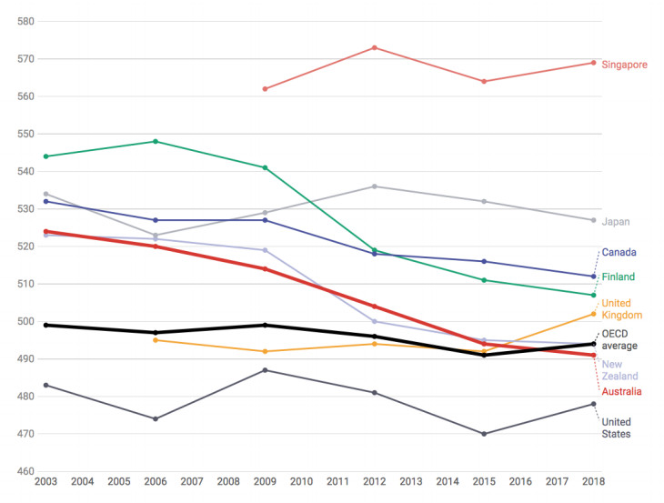
Programme for International Student Assessment (PISA) benchmark indicators (adapted from [11], p. 7)