Loading [MathJax]/jax/output/SVG/jax.js
Case study

Beyond the compass: Exploring geometric constructions via a circle arc template and a straightedge


  • Received: 01 January 2022 Revised: 01 February 2022
  • For thousands of years, the compass-and-straightedge tools have dominated the learning and teaching of geometry. As such, these inherited, long-standing instruments have gained a lustre of naturalized pedagogical value. However, mounting evidence suggests that many learners and teachers struggle to efficiently, effectively and safely use compasses when constructing geometric figures. Compasses are difficult for learners to use, can lead to inaccurate drawings, and can be dangerous. Thus, there is value in reconsidering the role of the compass in the learning and teaching of geometric constructions and to offer better tools as alternatives. The purpose of this work is to address the aforementioned need by proposing an alternative tool to the compass that is safer, more efficient and more effective. We will argue that a circle arc template forms such an alternative tool, and we will illustrate how learners and teachers can add value to their classrooms by using it, in conjunction with a straightedge, to establish the well-known constructions seen in geometry curricula around the world.

    Citation: Christopher C. Tisdell, David Bee Olmedo. Beyond the compass: Exploring geometric constructions via a circle arc template and a straightedge[J]. STEM Education, 2022, 2(1): 1-36. doi: 10.3934/steme.2022001
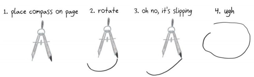
    Related Papers:

    [1] Lijing Ma, Shiru Qu, Lijun Song, Junxi Zhang, Jie Ren . Human-like car-following modeling based on online driving style recognition. Electronic Research Archive, 2023, 31(6): 3264-3290. doi: 10.3934/era.2023165
    [2] Pinglan Wan . Dynamic behavior of stochastic predator-prey system. Electronic Research Archive, 2023, 31(5): 2925-2939. doi: 10.3934/era.2023147
    [3] Yanjiao Li, Yue Zhang . Dynamic behavior on a multi-time scale eco-epidemic model with stochastic disturbances. Electronic Research Archive, 2025, 33(3): 1667-1692. doi: 10.3934/era.2025078
    [4] Yang Song, Beiyan Yang, Jimin Wang . Stability analysis and security control of nonlinear singular semi-Markov jump systems. Electronic Research Archive, 2025, 33(1): 1-25. doi: 10.3934/era.2025001
    [5] Ramalingam Sakthivel, Palanisamy Selvaraj, Oh-Min Kwon, Seong-Gon Choi, Rathinasamy Sakthivel . Robust memory control design for semi-Markovian jump systems with cyber attacks. Electronic Research Archive, 2023, 31(12): 7496-7510. doi: 10.3934/era.2023378
    [6] Yuan Tian, Jing Zhu, Jie Zheng, Kaibiao Sun . Modeling and analysis of a prey-predator system with prey habitat selection in an environment subject to stochastic disturbances. Electronic Research Archive, 2025, 33(2): 744-767. doi: 10.3934/era.2025034
    [7] Xinling Li, Xueli Qin, Zhiwei Wan, Weipeng Tai . Chaos synchronization of stochastic time-delay Lur'e systems: An asynchronous and adaptive event-triggered control approach. Electronic Research Archive, 2023, 31(9): 5589-5608. doi: 10.3934/era.2023284
    [8] Meng Gao, Xiaohui Ai . A stochastic Gilpin-Ayala nonautonomous competition model driven by mean-reverting OU process with finite Markov chain and Lévy jumps. Electronic Research Archive, 2024, 32(3): 1873-1900. doi: 10.3934/era.2024086
    [9] Chuntian Wang, Yuan Zhang . A multiscale stochastic criminal behavior model under a hybrid scheme. Electronic Research Archive, 2021, 29(4): 2741-2753. doi: 10.3934/era.2021011
    [10] Jiaqi Chang, Xiangxin Yin, Caoyuan Ma, Donghua Zhao, Yongzheng Sun . Estimation of the time cost with pinning control for stochastic complex networks. Electronic Research Archive, 2022, 30(9): 3509-3526. doi: 10.3934/era.2022179
  • For thousands of years, the compass-and-straightedge tools have dominated the learning and teaching of geometry. As such, these inherited, long-standing instruments have gained a lustre of naturalized pedagogical value. However, mounting evidence suggests that many learners and teachers struggle to efficiently, effectively and safely use compasses when constructing geometric figures. Compasses are difficult for learners to use, can lead to inaccurate drawings, and can be dangerous. Thus, there is value in reconsidering the role of the compass in the learning and teaching of geometric constructions and to offer better tools as alternatives. The purpose of this work is to address the aforementioned need by proposing an alternative tool to the compass that is safer, more efficient and more effective. We will argue that a circle arc template forms such an alternative tool, and we will illustrate how learners and teachers can add value to their classrooms by using it, in conjunction with a straightedge, to establish the well-known constructions seen in geometry curricula around the world.


    With the rapid increase of car occupancies, traffic congestion is becoming more and more serious, leading to tremendous environmental pollution and economic losses. Researchers have proposed many traffic flow models to study the mechanism behind complex traffic phenomena and provide a myriad of solutions to solve practical traffic problems. Among them, the car-following model offers an effective way to understand the mechanism of various complex traffic phenomena (such as traffic oscillation) from the perspective of individual interactions at the microscopic level. In 1961, Newell [1] proposed a car-following model that takes the optimal velocity into account and aligned with the experimental data of the steady flow. In 1995, Bando et al. [2] put forward an optimal velocity model (OVM), which successfully reproduced the evolution process for traffic congestion and received significant attention from many researchers later. However, the OVM may generate unrealistic values of acceleration and deceleration. To overcome this problem, Helbing and Tilch [3] proposed a generalized force model (GFM), which has a better fit with field data. GFM only considered the influence of a negative velocity difference on acceleration. In 2001, Jiang et al. [4] proposed the full velocity difference model (FVDM), considering negative and positive velocity differences.

    Based on those classical car-following models, many extended models were proposed by considering different factors from various perspectives. Yu and Shi [5] introduced the changes of multiple preceding cars' velocity with memory and formulated a new connected cruise control strategy, improving traffic safety and reducing fuel consumption. Chen et al. [6] proposed an extended OVM by considering multi-anticipative optimal velocity. The vehicle's acceleration was described as a function of the optimal velocity and desired distance to improve traffic flow stability. Based on the FVDM, the driver's backward-looking effect and traffic interruption probability were both integrated into the car-following model at the same time to enhance traffic flow stability effectively [7]. Considering the influence of the driver's memory, Tang et al. [8] and Liu et al. [9] proposed extended car-following models and illustrated that the driver's memory positively affected traffic flow stability. Apart from the above studies, many scholars [10,11,12,13,14,15,16,17,18,19,20] have also enriched the research in this field. Furthermore, the distribution of the driver's memory was considered, making the simulation results of car-following models closer to the empirical results [21,22]. Hossain et al. [23] redefined the backward-looking effect by proposing a positive backward equilibrium speed function based on the perspective of mathematical and physical theories, which strengthened the stability of traffic flow.

    With the emergence of advanced technologies, vehicle-to-vehicle (V2V) and vehicle-to-infrastructure (V2I) communication have great potential to mitigate traffic congestion and improve traffic safety. Jia and Ngoduy [24] incorporated V2V and V2I information into the following model and investigated the effects on driver behavior and traffic stability. Xiao et al. [25] proposed an expanded non-lane-based FVDM based on V2V communication technology. Ngoduy [26] studied the stability of heterogeneous traffic flow in a connected environment and derived the string stability conditions of the traffic flow. Larsson et al. [27] proposed a pro-social control strategy for connected autonomous vehicles in a mixed traffic flow environment to mitigate traffic fluctuations caused by human-driven vehicles. Numerous studies [28,29,30,31,32,33,34] applied intelligent traffic systems to reduce the instability of traffic flow by incorporating more dynamic traffic information into car-following models. Furthermore, Wu and Qu [35] discussed the positive role of connected technology in improving traffic flow efficiency and reducing energy consumption. Olovsson et al. [36] investigated the communication demands, privacy and network security issues of connected vehicles. In the meantime, the construction of the commercial data platform and infrastructure of connected vehicles has also been advancing [37].

    Up to now, studies on deterministic car-following models have made tremendous achievements. Yet, the deterministic car-following models cannot delineate the uncertainty of the driver's perception and behavior [38]. In fact, the driver's stochastic nature is one of the important causes of traffic oscillation. Previous experiments [38,39,40,41,42,43,44] indicated that standard deviations of the velocity increase in a concave way along with the platoon, which is obviously inconsistent with conventional car-following models. Therefore, a few scholars are devoted to developing stochastic car-following models to capture the stochasticity of drivers. Laval et al. [45] proposed a parsimonious stochastic car-following model by adding white noise to the driver's expected acceleration in free flow. The results show that the model can produce traffic oscillations that are consistent with the observation results. Yuan et al. [46] developed a geometric Brownian-motion car-following model to explain the capacity drop. Based on the experimental data, Tian et al. [43] found that the growth of velocity difference oscillation follows the mean reversion process, and then they proposed a mode-switching stochastic car-following model. In addition, they also investigated the car-following behavior from the perspective of wave travel time and proposed a simple stochastic car-following model based on the Newell model [47]. Ngoduy et al. [38] modeled the driver's acceleration process as an extended Cox–Ingersoll–Ross stochastic process and derived the stability conditions of the stochastic car-following model for the first time. Furthermore, by introducing the stochasticity of drivers into the macroscopic traffic flow model, Ngoduy [48] proposed a class of stochastic high-order continuous traffic flow models and analyzed the stability of traffic flow under the influence of noise.

    Although many researchers are devoted to capturing the driver's stochastic behavior by adding white noise to the acceleration function [38,45,46]; it does not reflect the relationship between stochasticity and some internal attributes of drivers (for example, some expectations or wishes of the driver during driving, which have a great impact on the driver's behavior and activities [49]); that is, the added white noise does not depend on some internal characteristics of the driver. However, Wagner [50,51] asserted that the random fluctuation of traffic flow is determined by the internal stochasticity of the driver itself. In addition, Makridis et al. [52] pointed out that the variation of the driver's desired velocity significantly impacts traffic flow stability. Therefore, it will be an interesting question of how the stochasticity of the driver's desired velocity influences the traffic flow stability.

    To better describe the impact of the driver's internal stochasticity on car-following behavior, we use stochastic progress to describe the stochastic property of the driver's desired velocity and propose a stochastic FVDM (SFVDM). Furthermore, we propose a stable speed guidance model (S-SFVDM) based on the V2I environment. The driver's memory effect is considered to alleviate the traffic oscillation caused by driving stochasticity. We derive the stochastic stability conditions for the proposed models based on the stochastic differential equation. We prove that the S-SFVDM can rapidly enhance traffic stability by finding the close equilibrium position based on the stochastic stability diagram regarding the current state of instability.

    The organization of the rest of this paper is as follows. Section 2 describes the formulation of the SFVMD and S-SFVDM. Section 3 derives the stochastic linear stability condition of two proposed models based on the Lyapunov stability analysis theory. In Section 4, numerical simulations are presented to verify the effectiveness of the developed models. Finally, the conclusions are summarized in Section 5.

    The desired velocity of the driver, which has proved to have a significant impact on the stability of traffic flow, is affected by the inherent attributes of the driver, and it is closely related to the driver's age, personality, environment and other complex factors. Therefore, the driver's desired velocity is not a fixed value, but fluctuates randomly in a bounded range over time. It is one of the internal stochasticity of drivers. Hence, in this paper, the driver's desired velocity is considered as a stochastic process rather than assuming a constant value. Similarly, our model is based on the classical FVDM, which is given by

    dvn(t)dt=α[Vop(xn(t))vn(t)]+λvn(t) (1)

    where vn(t) is the nth vehicle's velocity at time t. vn(t)=vn1(t)vn(t) and xn(t)=xn1(t)xn(t) are the velocity difference and distance between the nth vehicle and the (n-1)th vehicle at time t, respectively. α,λ are the headway sensitivity coefficient and the velocity difference sensitivity coefficient of the driver, respectively. V(xn(t)) is the optimal velocity (OV) function, given by [38]:

    Vop(xn(t))=v02[tanh(xn(t)h0a)+tanh(a)] (2)

    where v0 is the desired velocity of the driver, h0 is the critical headway and a is a positive constant.

    Yet, in reality, the desired velocity of a driver is not a constant, but fluctuates randomly in a bounded range over time with the dynamic variety of the driver's physiological and psychological properties. And, those properties are influenced by the external environment and many complex factors. To study the impact of the random variation of the desired velocity during stable traffic flow, we give the deterministic speed v0 a stochastic term. Without losing generality, we propose the extended OV function as follows:

    VSop(xn(t))=vSd2×[tanh(xn(t)h0a)+tanh(a)] (3)

    where vSd is the stochastic desired velocity, which is calculated as v0+ξ(xn(t),γ(t),vn(t)). ξ() is the stochastic source, which depends not only on the state of the vehicle, but also on the stochastic progress γ(t) at time t. When ξ()=0, VSop(xn(t))=Vop(xn(t)), which degenerates into Bando's OV function [3]. By taking the stochastic part ξ() into account in the FVDM, we develop the SFVDM, in which the Gaussian white noise is applied. By replacing Vop(xn(t)) with VSop(xn(t)) in Eq (1), we can reformat the SFVDM as

    dvn(t)=α[Vop(xn(t))vn(t)]dt+λvn(t)dt+αf(xn(t))1v0Vop(xn(t))dW(t) (4)

    where W(t) is a Wiener process. f(xn(t)) is the diffusion coefficient function of the stochastic term, which indicates that the strength of the stochasticity depends on the value of the headway. According to the actual situation, we could know that when the headway is large, the driver will show a high degree of stochasticity, because the random fluctuation of headway does not affect driving safety. On the contrary, when the headway is very small, drivers will drive carefully, so their stochasticity will remain at a low level. Hence, in this study, we consider the diffusion coefficient function f(xn(t)) of the stochastic term as follows:

    f(xn(t))=σtanh(xn(t)h0) (5)

    Equation (5) endows the model with a good characteristic. Previous studies [39,40,41,42,43,44] suggested that there is no unique relationship between the space headway and the vehicle's velocity. In other words, drivers do not maintain a fixed space headway at a certain velocity, as they randomly change their preferred space headway [40,41,42]. In reality, we know that the smaller the space headway, the more cautious the driver will become. With the space headway increasing, drivers may have the opportunity to elevate the desired velocity. In Eq (5), if the spacing is far less than the safe distance (i.e., xn(t)h0), tanh(xn(t)h0) will become very small. Hence, f(xn(t)) will be minimally affected by the high value of the constant σ. In other words, the impact of the stochastic part on the desired velocity will be reduced largely in this situation.

    Note that there is no consistent form of the diffusion coefficient function (i.e., Eq (5)) in previous studies [38,39,40,41,42,43,44,46,50], and it rarely affects the operation of vehicles [53]. On the one hand, the diffusion coefficient function developed in this paper guarantees a more reasonable acceleration with stronger non-negativity by integrating the driving state and traffic situation. On the other hand, it provides an opportunity to explore how the stochastic part in vSd influences traffic flow stability by deriving the string stability conditions.

    Equation (5) can also describe the driver's stochastic desired velocity characteristics when the headway is relatively large. Even if the headway is far greater than the safe distance (i.e., xn(t)h01), the oscillation of the stochastic part is bounded. The function term σtanh(xn(t)h0) can enhance the non-negativity of the velocity and ensure that negative values of velocity are not easily generated as in other stochastic car-following models [45,46].

    Stability analysis is an important part of traffic flow research [6,7,8,9,10,11,12]. The stochastic nature of each driver will influence the stability of traffic flow. In order to understand the impact of random changes in the driver's desired speed on the stability of traffic flow, this section focuses on the investigation of the linear stability condition of the SFVDM.

    Theoretically, each vehicle has the same velocity and space headway in the equilibrium state (vequ,xequ), given by v1=v2=v3==vequ and x1=x2=x3==xequ, where vequ=V(xequ). To derive the stability condition of the SFVDM, we put small disturbances (δvn(t)=vn(t)vequ and δxn(t)=xn(t)xequ) on the velocity and space headway around the equilibrium state, respectively. The first-order Taylor expansion is used to linearize the stochastically perturbed evolution equation as follows:

    δvn(t)=α[Vopδxn(t)δvn(t)]dt+λ(δvn1(t)δvn(t))dt+ασβδxn(t)dW(t) (6)

    where

    β=1v0(tanh(xequh0)Vop+Vop(xequ)h0(1tanh2(xequh0))) (7)

    In addition, the following equation could be obtained according to the definition and dynamics.

    dδxn(t)=[δvn1(t)δvn(t)]dt (8)

    A small disturbance may break the stable state of traffic flow under certain conditions and lead to local instability. The local stochastic stability analysis can help us understand the evolution of a small disturbance and how it leads to the local instability of the traffic flow. Based on the stochastic theory, the local stochastic stability condition is derived.

    To simplify the analysis of the proposed model, Equations (6) and (8) can be formulated as a matrix equation, as follows:

    dX(t)=PX(t)dt+QX(t)dW(t) (9)

    where

    X(t)=[δxn(t)δvn(t)] (10)
    P=[01αVop(α+λ)] (11)
    Q=[00αβσ0] (12)

    Based on the Lyapunov stability theory [54,55], we have the definition below for studying the local stability of the SFVDM.

    Definition 1. The trivial solution of Eq (9) is pth-moment exponentially stable if there exist two constants c1,c2(0,+] and a Lyapunov function V(X(t)) that satisfy the following two conditions:

    c1|X(t)|pV(X(t))c2|X(t)|p (13)
    LV(X(t))<κV(X(t)),κ0 (14)

    Equations (13) and (14) are equivalent to the generally strict formulation, as follows:

    limtt1E|X(t)|p<0 (15)

    where

    LV(X(t))=VX(X(t))PX(t)+12trace[(QX(t))TVXX(X(t))QX(t)] (16)
    VX(X(t))=(V(X(t))δvn(t),V(X(t))δxn(t))T (17)
    VXX(X(t))=(2V(X(t))δvn(t)δvn(t)2V(X(t))δvn(t)δxn(t)2V(X(t))δxn(t)δvn(t)2V(X(t))δxn(t)δxn(t)) (18)

    Based on Definition 1, we have the following theorem:

    Theorem 1. The SFVD model is 2nd-moment exponentially stable if

    σ22(α+λ)Vαβ2 (19)

    Proof. Based on the Lyapunov stability theory, the Lyapunov function is set as

    V(X(t))=(XT(t)FX(t))p2 (20)

    According to the definition of LV(X(t)), if the matrix F is positive-definite, LV(X(t)) can be reformatted as

    LV(X(t))=p(X(t)TFX(t))p21(X(t)TFPX(t))+p(p2)2(X(t)TFX(t))p22|(QX(t))TGQX(t)|2+12trace((QX(t))TFQX(t)) (21)

    Then, we set p=2, κ=0 and F as follows:

    F=[αV+12(α+λ)2(α+λ)2(α+λ)21] (22)

    The Lyapunov function is

    V(X(t))=[αV+12(α+λ)2]δxn2(t)(α+λ)δxn(t)δvn(t)+δvn2(t) (23)

    Furthermore,

    LV(X(t))=[α2β2σ2(α+λ)αV]δ2xn(t)(α+λ)2δ2vn(t) (24)

    If LV(X(t))0, Equation (14) holds. Equation (13) is also satisfied by setting the values of c1 and c2 as follows:

    c1=12(αV+12(α+λ)2+1)24[αV+14(α+λ)2]+12(αV+12(α+λ)2+1) (25)
    c2=12(αV+12(α+λ)2+1)24[αV+14(α+λ)2]+12(αV+12(α+λ)2+1) (26)

    The string stability analysis of the SFVDM explains how a small disturbance propagates from the first leading vehicle to the last vehicle in a platoon. If the string stability condition is satisfied, any small disturbance will be weakened from the leading vehicle to the next following vehicle and the strength of random fluctuations will be decreased continuously in traffic flow.

    We expand δvn(t)=ζ1einω+zt and δxn(t)=ζ2einω+zt in Eq (6), where ζ1 and ζ2 are two constants. Then, the SFVDM can also be treated as the linear stochastic ordinary difference equation:

    dX(t)=˜PX(t)dt+QX(t)dW(t) (27)

    where

    ˜P=[0eiω1αVαλ+λeiω] (28)

    To study the string stability of the proposed stochastic car-following model, Theorem 2 is given to study the moment exponential stability of the traffic flow.

    Theorem 2. The stochastic car-following model is 2nd-moment exponentially stable if

    σ2<2[α+λλ2+2αVop]α2β2 (29)

    Proof. According to Definition 1, by incorporating Eq (27) into Eq (21) and setting p=2, we can obtain the characteristic equation of the system as follows:

    z2z[α+λ(eiω1)+0.5α2β2σ2]αV(eiω1)=0 (30)

    Expanding z=iωz1+ω2z2+ into Eq (30) and ignoring the high-order terms, the expressions of z1 and z2 can be obtained as follows by setting the first-order and second-order terms to be zero:

    z1=αVopα12α2β2σ2 (31)
    z2=z21+λz112αVα12α2β2σ2 (32)

    The condition of stochastic stability will be held if z1<0 and z2<0. Hence, we can obtain the stability conditions by treating σ as the variable:

    σ2<2[α+λλ2+2αVop]α2β2 (33)

    It is worth mentioning that, if σ=0, the SFVDM will degenerate to the FVDM. In the meantime, the stochastic stability condition will become Vop<α2+λ, which is the stability condition of the FVDM.

    Figure 1 shows the stability diagrams for the SFVDM with different values of the velocity difference sensitivity coefficient λ, where the values of λ in Figure 1(a)(d) are 0.24, 0.28, 0.32 and 0.36, respectively. Other parameters of the SFVDM were set as α=0.3s1, h=2m and Vexp=2m/s. In Figure 1, it is shown that the coverage of the unstable region decreases as the value of λ increases.

    Figure 1.  Stability region of SFVDM with different values of λ, where (a) λ=0.24, (b)λ=0.28, (c) λ=0.32 and (d) λ=0.36.

    Figure 2 shows the stability diagrams for the FVDM. Note that Figure 1d and Figure 2 have the same value of λ (i.e., λ=0.36). In Figure 2, the traffic flow is always in a stable state when α>0.28. In Figure 1(d), the traffic flow is in the stable regime when σ<1.2, but it is always in the unstable region when σ>1.2. It clearly indicates that the stochasticity has a significant potential negative impact on the stability of traffic flow. When the random noise strength exceeds a threshold value, the traffic flow will become unstable. In addition, when λ is a relatively small value (e.g., λ<0.32), a small value of σ will result in instability of the traffic flow with headways between 3.5 and 4 m. It indicates that the driver's stochasticity will decrease the stability of the traffic flow.

    Figure 2.  Stability region of FVDM.

    According to the above analysis, we can observe that the stochastic desired velocity of the driver is a critical factor that induces the instability of the traffic flow. This result is consistent with the findings in the previous study [52]. Therefore, it is necessary to design a control strategy to reduce the negative impacts of stochastic driving properties on the traffic flow. V2I communication technology can realize the information interaction between vehicles and roadside facilities within an effective range, which provides a prerequisite for speed guidance. In the next section, a stable speed guidance strategy is proposed considering the driver's memory effect, as based on the V2I environment, to address the above issue.

    The development of V2I communication technology allows us to alleviate the traffic oscillation caused by the driver's stochastic nature. In this section, we propose an S-SFVDM to reduce the effect of the driver's randomly desired velocity based on the V2I environment. We consider the potential influence of the driver's short-term memory on the speed guidance. We assume that all vehicles can communicate with the intelligent roadside system that can capture all vehicles' speeds, locations and other useful information at each time step (communication delay will not be considered in this study).

    Based on the stability diagram, it is easy to find the point e(ˉxt,σ) by fixing σ at any time step, where ˉxt denotes the mean value of the space headway of all vehicles at time t. The essential idea is that it is easy to find the equilibrium point e nearest to the current point e in the unstable region as the expected state for when the platoon will arrive after the speed guidance. And, this process is real-time and dynamic.

    The stable speed guidance strategy is described using the following equations:

    dvn(t)=α[Vop(xn(t))vn(t)]dt+λvn(t)dt+ασtanh(xn(t)h0)1v0Vop(xn(t))dW(t)+ϕ(η[g(ˉxt)τTsk=0fΓ(kτ)vn(tkτ)]+(1η)[g(ˉxt)τTsk=0fΓ(kτ)vn1(tkτ)]) (34)
    g(ˉxt)=VSop(ˉxt) (35)

    where ϕ denotes the mean value of the compliance of drivers to the speed guidance. η[0.5,1] indicates that the weight of the target vehicle in the speed guidance strategy is greater than the preceding vehicle. τ is the length of each memory interval. ϕ, τ and η are all constants. g(ˉxt) denotes the of guidance speed computed by the intelligent roadside system.

    The driver's memory effect is assumed to be homogeneous in many studies. It can potentially incur unrealistic phenomena. For example, when the length of the time period of the driver's historical memory is a relatively large value, the car-following system will be stable regardless of the value of the sensitivity. One reason leading to this problem is that the memory effect of drivers should decay to zero when the time increases to a large value. In order to better describe the actual situation, the memory effect of drivers is considered as a gamma distribution [21,22] in this paper.

    fΓ(ω)=umωm1euωΓ(u) (36)
    Γ(u)=+0xu1exdx (37)

    When a vehicle is in the steady state, under critical conditions, Equation (33) can be formulated as

    σ(Δx)=2αβα+λλ2+2αVop (38)

    The stability diagrams show that the function σ(Δx) is monotonic both in the left part and the right part. It is decreasing in the left parts and increasing in the right parts. Figure 3 gives the sketch map of the stable speed guidance strategy based on the stable diagram. The intention for this study was to identify a reasonable and effective guidance velocity which can facilitate the process of stabilizing traffic flow. More specifically, we first calculate the average headway Δˉx of traffic flow and find the point et(Δˆx,σt), which is the closest position of the stable regime to et(Δˉx,σt) with a fixed σt. The expression of neutral stable curves C1 and C2 are already obtained so that we can derive the point et(Δˆx,σt) by calculating d1t and d2t(d1td2t). To calculate dit accurately, we use the simple least squares method to compute the intersection et(Δˆx,σt). The relationship between iteration error and iteration times is as follows:

    bupblow2jiter+1<ε (39)
    Figure 3.  Sketch map of stable speed guidance strategy based on the stable diagram in equilibrium space headway-diffusion coefficient space under the conditions of the V2I environment.

    where jiter is the number of iterations and ε is the iterative error.

    If there is a small deviation from the equilibrium state, the function g(ˉxt) could be treated as a constant. The stability analysis can be explored in this situation, as the results display how the speed guidance under the conditions of the V2I environment influence the stability of traffic considering driver memory. Therefore, in the next step, the stability analysis of the expanded stochastic model will be deduced. For simplicity, we give the stability condition directly by omitting the details here, and the detailed derivation process is given in Appendix A.

    The S-SFVDM is considered to be 2nd-moment exponentially stable if

    σ2<4(α+λ+ϕητTsk=0fΓ(kτ)[λϕ(1η)τTsk=0fΓ(kτ)]2+2(1ϕτ2Tsk=0kfΓ(kτ))αVop)α2β2 (40)

    Later, we will find that, compared with the SFVDM, the S-SFVDM has a larger stability region due to considering the speed guidance strategy.

    Figure 4 shows the neutral stability curves for different values of ϕ. The region enclosed by the curve and coordinate axis is the stable region of the traffic flow, and all other regions are the unstable region of the traffic flow. Figure 4 indicates that, with the increase of ϕ, the stability of the stochastic car-following model becomes stronger. It further indicates that providing effective speed guidance information to the driver, given that the driver's memory is considered, is beneficial to the improvement of the stability of traffic flow based on V2I technology. This result is consistent with many findings of relevant studies [21,22,23,24,25,26].

    Figure 4.  Stable diagram in equilibrium space headway-diffusion coefficient space for different values of ϕ.

    Figure 5 describes the neutral stability curves for different values of η. The region enclosed by the curve and coordinate axis is the stable region of the traffic flow, and all other regions are the unstable region of the traffic flow. It can be seen in Figure 5 that the stability of the traffic flow increases with the decrease of η, which indicates that considering the dynamics of the preceding vehicle for the target vehicle in the speed guidance strategy is conducive to improving the stability of the traffic flow. In addition, we can also find that a change in η has a limited impact on the stability of traffic flow.

    Figure 5.  Stable diagram in equilibrium space headway-diffusion coefficient space for different values of η(0.6,0.8,1.0).

    Figure 6 displays the stable diagram in equilibrium space headway-diffusion coefficient space for different values of Ts, where (a) λ=0.28,ϕ=0.03 and (b) λ=0.3,ϕ=0.02. The region enclosed by the curve and coordinate axis is the stable region of the traffic flow, and all other regions are the unstable region of the traffic flow. It indicates that the area of the stability region increases with increasing driver memory time. In addition, Figure 6 shows that the increase in the stability regime gradually converges with the elongation of the driver's memory time. Meanwhile, taking the driver's memory into account is more reasonable [21,22].

    Figure 6.  Stable diagram in equilibrium space headway-diffusion coefficient space for different values of Ts and different parameter settings, where (a) λ=0.28,ϕ=0.03 and (b) λ=0.3,ϕ=0.02.

    In order to validate the accuracy of the theoretical analysis and the superiority of the proposed models, numerical simulations were carried out under a periodic boundary condition. We assumed that all vehicles run on a ring road and have the same initial headway, as well as the same velocity. For simplicity, we applied the explicit Euler–Maruyama scheme to discretize the stochastic differential equation. The numerical approximation of the SFVDM is

    vn(k+1)vn(k)=α[Vop(Δxn(k))vn(k)]Δt+ασtanh(Δxn(k)h0)1v0Vop(Δxn(k))ΔtΔW(k+1)+λvn(k)Δt (41)

    Based on the proposed SFVDM, we first carried out a series of simulations of platoon with different numbers of vehicles under the open boundary condition (i.e., on a straight road of infinite length). The model parameters were as follows:

    α=0.3,λ=0.3,h0=15m,v0=20m/s,σ=1 (42)

    The standard deviations of the speed profiles and fitting curves of different simulations are shown in Figure 7. The number of vehicles in each sub-figure are (a) 50 vehicles, (b) 100 vehicles, (c) 150 vehicles and (d) 200 vehicles. In Figure 7, the black points represent the standard deviation of each vehicle's velocity in the platoon, and the blue lines are quadratic polynomial fitting curves in different simulations. Figure 7 shows an interesting property of the SFVDM, where the profiles of the standard deviations of speed are concave curves, which are consistent with empirical data [38,39,40,41,42,43,52].

    Figure 7.  Standard deviations of speed profiles and fitting curves for different simulated numbers of vehicles, where (a) 50 vehicles, (b) 100 vehicles, (c) 150 vehicles and (d) 200 vehicles.

    To further verify the SFVDM and S-SFVDM, we conducted a series of simulations under the periodic boundary condition (i.e., on a ring road). The initial parameters are given as follows: the vehicle number N=100, the road length L=400m and the time step of the simulation was 0.1 s. Other parameters were set as follows:

    α=0.3,λ=0.3,η=0.7,h0=2m,v0=2m/s,a=2,t=3000s (43)
    x1(0)=LLN (44)
    xn(0)=(Nn)LN(n=2,3,4,,N) (45)
    v1(t)=v2(t)==vn(t)=ve=Vop(LN) (46)
    v1(20/τ)=0.9ve (47)

    Figure 8 shows the time-space evolutions of the platoon for different values of the diffusion coefficient σ=0,0.5,1,1.5, with the color representing vehicle velocity. From Figure 8, it can be found that, with the increase of σ, the oscillation of velocity becomes larger. In addition, higher stochasticity leads to more vehicles staying at a low-velocity state for a longer period. It indicates that the increasing stochasticity of drivers leads to stronger instability of traffic flow and more frequent stop-and-go phenomena. Furthermore, with the increase in the intensity of the randomness of the driver's desired velocity, the density wave of traffic flow becomes more uneven.

    Figure 8.  Time-space evolutions of all vehicles for different values of σ, where (a)σ=0, (b) σ=0.5, (c) σ=1 and (d) σ=1.5.

    Figure 9 shows the time-space evolutions of the headway profile for different values of σ. In Figure 9, λ is equal to 3.0, and the headway is equal to 3.2 m. According to Theorem 2, the boundary of stability is 2<σ=2.276<2.5. In Figure 9(a), large uneven oscillations occur in the headway and the traffic flow is extremely unstable. On the contrary, the headway is steady without fluctuation in Figure 9(b), and the traffic flow is stochastically stable. The simulation results are consistent with the stability boundary conditions.

    Figure 9.  Time-space evolutions of the headway profile after a sufficient time t=1400s, where (a) σ=2.5 and (b) σ=2.0.

    Figure 10 shows the snapshots of the headway configuration of all vehicles at time t=1650s for different values of σ. It shows that the headway oscillations in Figure 10(a) are severe. However, the headway profile in Figure 10(b) approximates a straight line. Similarly, we also verify the correctness of the stability condition under another condition.

    Figure 10.  Snapshots of headway configuration of all vehicles at time t=1650s, where (a) σ=2.5 and (b) σ=2.0.

    As shown in Figures 11 and 12, the time-space evolutions of the headway profile and snapshots of the headway configuration of all vehicles at time t=2650s were both used to further test the correctness of the stability conditions. According to Eq (33), when λ=0.36 and the headway is equal to 3.8 m, the stable boundary condition is 1<σ=1.528<2. It indicates that the traffic flow is unstable when σ=2, and that the traffic flow is in the string stability regime when σ=1, which are in line with the numerical simulation results revealed in Figures 11 and 12. Moreover, these results suggest that the driver's stochastically desired velocity will decrease the stability of traffic flow. However, with the increase of the stochasticity strength, the stable regime will further reduce and the oscillation of traffic flow tends to become more serious. Therefore, the random variation of the driver's desired velocity is one of the important reasons for traffic oscillation.

    Figure 11.  Time-space evolutions of the headway profile after a sufficient time t=2300s, where (a) σ=2.0 and (b) σ=1.0.
    Figure 12.  Snapshots of headway configuration of all vehicles at time t=2650s, where (a) σ=2.0 and (b) σ=1.0.

    Figure 13 presents the time-space evolutions of the headway profiles for ϕ=0.00,0.01,0.02,0.03. Drivers do not receive the speed guidance information when ϕ=0. The amplitude of the headway profile is considerable and traffic flow is volatile. With the increase of ϕ, the amplitude of the headway profile decays obviously. It indicates that the fluctuation of traffic flow decreases with the increase of ϕ. When ϕ=0.03, the traffic flow is stochastically stable. Figure 14 shows snapshots of the headway configuration of all vehicles at time t=2350s for different values of ϕ, which shows the same results as Figure 13.

    Figure 13.  Time-space evolutions of the headway profiles for different values of ϕ, where (a) ϕ=0.00, (b) ϕ=0.01, (c) ϕ=0.02 and (d) ϕ=0.03.
    Figure 14.  Snapshots of headway configuration of all vehicles at time t=2350s for different values of ϕ, where (a) ϕ=0.00, (b) ϕ=0.01, (c) ϕ=0.02 and (d) ϕ=0.03.

    Meanwhile, we can conclude from the above diagrams that giving equilibrium speed guidance to the driver can effectively reduce the instability of traffic flow caused by the random change of the driver's desired velocity. Compared with the SFVDM, the proposed S-SFVDM based on the V2I environment has a larger stable region. Moreover, the negative impact of the stochasticity of the driver's desired velocity can be abated effectively by stable speed guidance. The numerical simulation results are consistent with the theoretical analysis results.

    In this study, a stochastic car-following model, i.e., an SFVDM, was developed to explore the impact of human expectation uncertainty of velocity on traffic stability. The desired velocity of the driver was considered as a stochastic process. The magnitude of the stochasticity is related to the traffic condition, which determines the non-negativity of the vehicle's velocity in most cases. Stochastic stability analysis was simulated to observe the conditions of local stability and string stability of traffic flow. The results demonstrate that the driver's stochastic desired velocity will decrease the coverage of the stable regime. To reduce the negative effects of the internal stochasticity of the driver, we developed a stable speed guidance strategy, i.e., the S-SFVDM, based on the V2I environment. Furthermore, the driver's memory effect is considered as a gamma distribution to fit the actual situation better. Numerical simulations were carried out to validate the proposed models. The results indicate that the stability of traffic flow can be enhanced effectively by applying the proposed stable speed guidance strategy. Specifically, sending a stable guidance velocity to each driver can weaken the negative influence brought about by the driver's stochastic nature.

    However, the main work of this paper focuses on the model formulation and the derivation of the stochastic stability analysis of the proposed model. The model parameters were not calibrated based on field or experimental data. In future research, we will conduct car-following experiments to validate the numerical results and calibrate the model parameters. In addition, modeling and analysis of heterogeneous traffic flow that mixes regular and connected vehicles with the stochastic nature of humans are also further research directions.

    This work was supported by the National Natural Science Foundation of China (72201010) and the China Postdoctoral Science Foundation (2021M700304).

    The authors declare that there is no conflict of interest.

    Expand δvn(t)=ζ1einω+zt and δxn(t)=ζ2einω+zt. ζ1 and ζ2 are constants. Therefore, Equation (34) can be read as the linear stochastic ordinary differential equation:

    dX(t)=PSGX(t)dt+QSGX(t)dW(t) (A1)

    where

    PSG=[0eiω1αVα+λ(eiω1)+ρ(λ,k,τ,η,ϕ)] (A2)
    QSG=[00ασβ0] (A3)
    ρ(k,τ,η,φ)=ϕτηTsk=0fΓ(kτ)ezkτ+ϕτ(1η)Tsk=0fΓ(kτ)eiωzkτ (A4)

    Based on Definition 1, Theorem 3 and the corresponding proof will be derived.

    Theorem 3. The stochastic car-following model with the speed guidance strategy considered is 2nd-moment exponentially stable if

    σ2<4(α+λ+ϕητTsk=0fΓ(kτ)[λϕ(1η)τTsk=0fΓ(kτ)]2+2(1ϕτ2Tsk=0kfΓ(kτ))αVop)α2β2 (A5)

    where Ts=T/τ.

    Proof. The characteristic equation of the matrix P is

    z2z(α+λ(eiw1)+ϕτ[ηTsk=0fΓ(kτ)eλiτ+(1η)Tsk=0fΓ(kτ)eiωλkτ])αV(eiω1)=0 (A6)

    Expanding z=iωz1+ω2z2+ into Eq (A6) and ignoring the high-order terms by setting the first-order and second-order terms to zeros, the expressions of z1 and z2 can be obtained:

    z1=αVα+ϕτTsk=0fΓ(kτ)12α2β2σ2 (A7)
    (1ϕτ2Tsk=0kfΓ(kτ))(αVα+ϕτTsk=0fΓ(kτ)12α2β2σ2)2+[λϕ(1η)τTsk=0fΓ(kτ)](αVα+ϕτTsk=0fΓ(kτ)12α2β2σ2)+12αVα+ϕτTsk=0fΓ(kτ)12α2β2σ2 (A8)

    The condition of stochastic stability will be held only if z1<0 and z2<0. Therefore, we can obtain the stability conditions by taking σ as the variable:

    σ2<4(α+λϕητTsk=0fΓ(kτ)[λϕ(1η)τTsk=0fΓ(kτ)]2+2(1ϕτ2Tsk=0kfΓ(kτ))αVop)α2β2 (A9)

    When τTsk=0fΓ(kτ)1 (for example, Ts>100=10s and τTsk=0fΓ(kτ)1 for u=2 and m=1; 10 s was deemed as a reasonable value of the length of effective memory time of drivers [18]), Equation (A9) can be simplified as

    σ2<4(α+λϕη[λϕ(1η)]2+2(1ϕτ2Tsk=0kfΓ(kτ))αVop)α2β2 (A10)


    [1]

    Department of Education. Mathematics programmes of study: Key stage 3. National curriculum in England. Document DFE-00179-2013. 2013; Available from: https://assets.publishing.service.gov.uk/government/uploads/system/uploads/attachment_data/file/239058/SECONDARY_national_curriculum_-_Mathematics.pdf.

    [2]

    Common Core State Standards Initiative. High School: Geometry - Congruence- Make Geometric Constructions.; Available from: http://www.corestandards.org/Math/Content/HSG/CO/#CCSS.Math.Content.HSG.CO.D.12.

    [3]

    Assessment and Reporting Authority [ACARA] Australian Curriculum. F-10 Australian Mathematics Curriculum-Mathematics (Version 8.4). 2021; Available from: https://www.australiancurriculum.edu.au/f-10-curriculum/mathematics/?year=11758&strand=Measurement+and+Geometry&elaborations=true&elaborations=false&scotterms=false&isFirstPageLoad=false.

    [4]

    Ministry of Education Singapore. MATHEMATICS SYLLABUSES. Secondary One to Four. Express Course. Normal (Academic) Course. 2019; Available from: https://www.moe.gov.sg/-/media/files/secondary/syllabuses/maths/2020-express_na-maths_syllabuses.pdf?la=en&hash=95B771908EE3D777F87C5D6560EBE6DDAF31D7EF.

    [5]

    NZMaths. Ruler and Compass Constructions. 2021; Available from: https://nzmaths.co.nz/resource/ruler-and-compass-constructions.

    [6]

    Martin, G.E., Geometric constructions. 1998, New York: New York : Springer.

    [7]

    Brown, P., Evans, M., Hunt, D., McIntosh, J., Pender, B., and Ramagge, J., Construction - Measurement and Geometry : Module 13, 2011, The University of Melbourne on behalf of the international Centre of Excellence for Education in Mathematics, Melbourne. Available from: http://amsi.org.au/teacher_modules/Construction.html.

    [8]

    Schaaf, W.L.E., Reprint Series: Mascheroni Constructions. RS-4. 1967, Stanford, California, USA: Stanford University.

    [9]

    Albrecht, W.A.J., A Critical And Historical Study Of The Role Of Ruler And Compass Constructions In The Teaching Of High School Geometry In The United States, PhD Thesis, 1952, The Ohio State University, Ann Arbor.

    [10]

    Hendroanto, A. and Fitriyani, H., Analyzing the need of math geometry drawing tools in mathematics classroom. Journal of Physics: Conference Series, 2019, 1188: 012051. https://doi.org/10.1088/1742-6596/1188/1/012051.

    doi: 10.1088/1742-6596/1188/1/012051
    [11]

    Orlin. B., Math with Bad Drawings- Compass Constructions Made Easy. 2018; Available from: https://mathwithbaddrawings.com/2018/01/10/compass-constructions-made-easy/.

    [12]

    Richeson, D.S., Tales of Impossibility - The 2000-Year Quest to Solve the Mathematical Problems of Antiquity. 2019: Princeton University Press.

    [13]

    Vernon, J., Student stabbed with compass, 2013, Hutt News, New Zealand, Available from: http://www.stuff.co.nz/dominion-post/news/local-papers/hutt-news/8865591/Student-stabbed-with-compass.

    [14]

    Jiang, E., Chinese teacher is detained after 'using a drawing compass to stab and injure dozens of students because they failed to finish their homework', 2020, Daily Mail Australia, Australia. Available from: https://www.dailymail.co.uk/news/article-8369935/Chinese-teacher-detained-using-compass-stab-dozens-students.html.

    [15]

    Bhattacharya, S., 14-year-old stabbed to death with compass 'over girl', 2017, The Times of India, India. Available from: https://timesofindia.indiatimes.com/city/delhi/14-yr-old-stabbed-to-death-with-compass-over-girl/articleshow/58466802.cms.

    [16]

    Welkowitz, S., Tenth Year Geometry for all American Youth. The Mathematics Teacher, 1946, 39(3): 99‒112. https://www.jstor.org/stable/27953069.

    [17]

    Day Ashley, L., Case Study Research, in Research Methods & Methodologies in Education, R. Coe, et al., Editors. 2017, pp. 114‒121. Los Angeles, CA: SAGE.

    [18]

    Dounskaia, N. and Goble, J.A., The role of vision, speed, and attention in overcoming directional biases during arm movements. Experimental Brain Research, 2011,209(2): 299‒309. https://doi.org/10.1007/s00221-011-2547-9.

    doi: 10.1007/s00221-011-2547-9
    [19]

    Dounskaia, N.V., Ketcham, C.J., and Stelmach, G.E., Influence of Biomechanical Constraints on Horizontal Arm Movements. Motor Control, 2002, 6(4): 366‒387. https://doi.org/10.1123/mcj.6.4.366.

    doi: 10.1123/mcj.6.4.366
    [20]

    Severi, F., Sui problemi determinati risolubili colla riga e col compasso (Estratto da una Lettera al Prof. F. Enriques). Rendiconti del Circolo matematico di Palermo, 1904, 18(1): 256‒259. https://doi.org/10.1007/BF03014102.

    doi: 10.1007/BF03014102
    [21]

    Steiner, J. and Archibald, R.C., Geometrical constructions with a ruler, given a fixed circle with its center. Scripta mathematica studies: no. 4. 1950: Scripta Mathematica, Yeshiva University.

    [22]

    Mackay, J.S., Solutions of Euclid's Problems, with a rule and one fixed aperture of the compasses, by the Italian geometers of the sixteenth century. Proceedings of the Edinburgh Mathematical Society, 1886, 5: 2‒22. https://doi.org/10.1017/S0013091500001334.

    doi: 10.1017/S0013091500001334
    [23]

    Gibb, A.A., There are more ways than one to bisect a segment. The Mathematics Teacher, 1977, 70(5): 390‒393. http://www.jstor.org/stable/27960865.

    [24]

    Hlavaty, J.H., Mascheroni constructions. The Mathematics Teacher, 1957, 50(7): 482‒487. http://www.jstor.org/stable/27955488.

  • This article has been cited by:

    1. Ying Luo, Yanyan Chen, Kaiming Lu, Liang Chen, Jian Zhang, Modeling and analysis of heterogeneous traffic flow considering dynamic information flow topology and driving behavioral characteristics, 2024, 637, 03784371, 129521, 10.1016/j.physa.2024.129521
    2. Congcong Bai, Jun Jing, Bokun Liu, Wenbin Yao, Chengcheng Yang, Adjé Jérémie Alagbé, Sheng Jin, Jose E. Naranjo, Exploring Heterogeneity in Car-Following Behaviors Based on Driver Visual Characteristics: Modeling and Calibration, 2023, 2023, 2042-3195, 1, 10.1155/2023/5583081
  • Reader Comments
  • © 2022 the Author(s), licensee AIMS Press. This is an open access article distributed under the terms of the Creative Commons Attribution License (http://creativecommons.org/licenses/by/4.0)
通讯作者: 陈斌, bchen63@163.com
  • 1. 

    沈阳化工大学材料科学与工程学院 沈阳 110142

  1. 本站搜索
  2. 百度学术搜索
  3. 万方数据库搜索
  4. CNKI搜索

Metrics

Article views(3121) PDF downloads(237) Cited by(0)

Figures and Tables

Figures(52)

Other Articles By Authors

/

DownLoad:  Full-Size Img  PowerPoint
Return
Return

Catalog