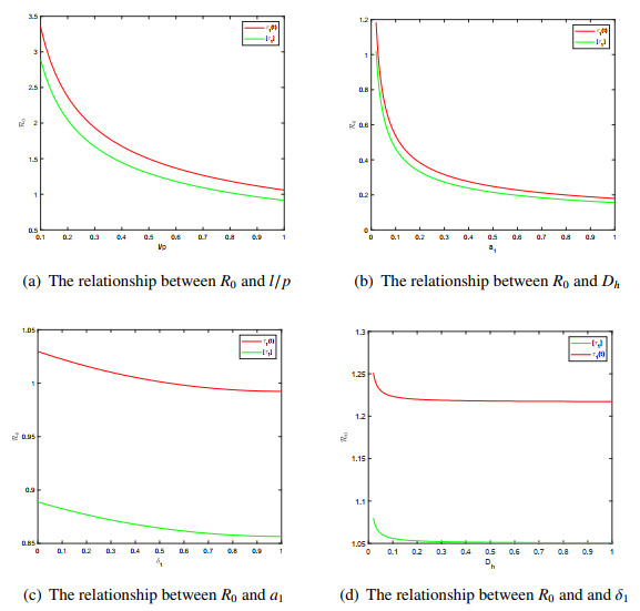
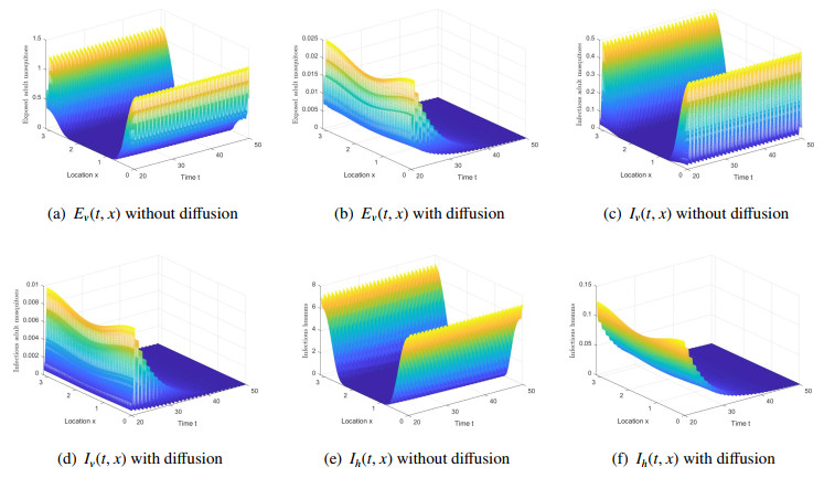
One of the most important vector-borne disease in humans is malaria, caused by Plasmodium parasite. Seasonal temperature elements have a major effect on the life development of mosquitoes and the development of parasites. In this paper, we establish and analyze a reaction-diffusion model, which includes seasonality, vector-bias, temperature-dependent extrinsic incubation period (EIP) and maturation delay in mosquitoes. In order to get the model threshold dynamics, a threshold parameter, the basic reproduction number $ R_{0} $ is introduced, which is the spectral radius of the next generation operator. Quantitative analysis indicates that when $ R_{0} < 1 $, there is a globally attractive disease-free $ \omega $-periodic solution; disease is uniformly persistent in humans and mosquitoes if $ R_{0} > 1 $. Numerical simulations verify the results of the theoretical analysis and discuss the effects of diffusion and seasonality. We study the relationship between the parameters in the model and $ R_{0} $. More importantly, how to allocate medical resources to reduce the spread of disease is explored through numerical simulations. Last but not least, we discover that when studying malaria transmission, ignoring vector-bias or assuming that the maturity period is not affected by temperature, the risk of disease transmission will be underestimate.
Citation: Hongyong Zhao, Yangyang Shi, Xuebing Zhang. Dynamic analysis of a malaria reaction-diffusion model with periodic delays and vector bias[J]. Mathematical Biosciences and Engineering, 2022, 19(3): 2538-2574. doi: 10.3934/mbe.2022117
One of the most important vector-borne disease in humans is malaria, caused by Plasmodium parasite. Seasonal temperature elements have a major effect on the life development of mosquitoes and the development of parasites. In this paper, we establish and analyze a reaction-diffusion model, which includes seasonality, vector-bias, temperature-dependent extrinsic incubation period (EIP) and maturation delay in mosquitoes. In order to get the model threshold dynamics, a threshold parameter, the basic reproduction number $ R_{0} $ is introduced, which is the spectral radius of the next generation operator. Quantitative analysis indicates that when $ R_{0} < 1 $, there is a globally attractive disease-free $ \omega $-periodic solution; disease is uniformly persistent in humans and mosquitoes if $ R_{0} > 1 $. Numerical simulations verify the results of the theoretical analysis and discuss the effects of diffusion and seasonality. We study the relationship between the parameters in the model and $ R_{0} $. More importantly, how to allocate medical resources to reduce the spread of disease is explored through numerical simulations. Last but not least, we discover that when studying malaria transmission, ignoring vector-bias or assuming that the maturity period is not affected by temperature, the risk of disease transmission will be underestimate.

| [1] | Centers for disease control and prevention. Available from: https://www.cdc.gov/malaria/malaria-worldwide/impact.html. |
| [2] |
R. Ross, An application of the theory of probabilities to the study of a priori pathometry, Part I, Proc. R. Soc. Lond. A, 92 (1916), 204–230. https://doi.org/10.1098/rspb.1917.0008 doi: 10.1098/rspb.1917.0008

|
| [3] | G. Macdonald, The analysis of equilibrium in malaria, Trop. Dis. Bull., 49 (1952), 813–829. |
| [4] |
S. Ruan, D. Xiao, J. C. Beier, On the delayed Ross-Macdonald model for malaria transmission, Bull. Math. Biol., 70 (2008), 1098–1114. https://doi.org/10.1007/s11538-007-9292-z doi: 10.1007/s11538-007-9292-z
|
| [5] |
T. J. Hagenaars, C. A. Donnelly, N. M. Ferguson, Spatial heterogeneity and the persistence of infectious diseases, J. Theor. Biol., 229 (2004), 349–359. https://doi.org/10.1016/j.jtbi.2004.04.002 doi: 10.1016/j.jtbi.2004.04.002
|
| [6] |
J. Ge, K. I. Kim, Z. Lin, H. Zhu, A SIS reaction-diffusion-advection model in a low-risk and high-risk domain, J. Differential Equations, 259 (2015), 5486–5509. https://doi.org/10.1016/j.jde.2015.06.035 doi: 10.1016/j.jde.2015.06.035
|
| [7] | V. Capasso, Mathematical structures of epidemic systems, Springer, 2008. |
| [8] |
J. Skellam, Random dispersal in theoretical populations, Biometrika, 38 (1951), 196–218. https://doi.org/10.1007/BF02464427 doi: 10.1007/BF02464427
|
| [9] | J. D. Murray, Mathematical Biology, Springer-Verlag, 1989. |
| [10] |
D. L. Smith, N. Ruktanonchai, Progress in modelling malaria transmission, Adv. Exp. Med. Biol., 673 (2010), 1–12. https://doi.org/10.1007/978-1-4419-6064-1_1 doi: 10.1007/978-1-4419-6064-1_1
|
| [11] |
S. Mandal, R. R. Sarkar, S. Sinha, Mathematical models of malaria-a review, Malaria J., 10 (2011), 202. https://doi.org/10.1186/1475-2875-10-202 doi: 10.1186/1475-2875-10-202
|
| [12] |
R. Lacroix, R. W. Mukabana, L. C. Gouagna, J. C. Koella, Malaria infection increases attractiveness of humans to mosquitoes, PLoS Biol., 3 (2005), e298. https://doi.org/10.1371/journal.pbio.0030298 doi: 10.1371/journal.pbio.0030298
|
| [13] |
F. Chamchod, N. F. Britton, Analysis of a vector-bias model on malaria transmission, Bull. Math. Biol., 73 (2011), 639–657. https://doi.org/10.1007/s11538-010-9545-0 doi: 10.1007/s11538-010-9545-0
|
| [14] |
S. Kim, M. A. Masud, G. Cho, I. H. Jung, Analysis of a vector-bias effect in the spread of malaria between two different incidence areas, J. Theor. Biol., 419 (2017), 66–76. https://doi.org/10.1016/j.jtbi.2017.02.005 doi: 10.1016/j.jtbi.2017.02.005
|
| [15] |
B. Buonomo, C. Vargas-De-León, Stability and bifurcation analysis of a vector-bias model of malaria transmission, Math. Biosci., 242 (2013), 59–67. https://doi.org/10.1016/j.mbs.2012.12.001 doi: 10.1016/j.mbs.2012.12.001
|
| [16] |
E. N. Osman, J. Li, Analysis of a vector-bias malaria transmission model with application to Mexico, Sudan and Democratic Republic of the Congo, J. Theor. Biol., 2019, 72–84. https://doi.org/10.1016/j.jtbi.2018.12.033 doi: 10.1016/j.jtbi.2018.12.033
|
| [17] | P. Jones, C. Harpham, C. Kilsbyet, Projections of future daily climate for the UK from the weather generator, UK climate projections science report, 2009. |
| [18] |
A. T. Ciota, A. C. Matacchiero, K. A. Marm, L. D. Kramer, The effect of temperature on life history traits of Culex mosquitoes, J. Med. Entomol., 51 (2014), 55–62. https://doi.org/10.1603/ME13003 doi: 10.1603/ME13003
|
| [19] |
Y. Lou, X. Q. Zhao, A climate-based malaria transmission model with structured vector population, SIAM J. Appl. Math., 70 (2010), 2023–2044. https://doi.org/10.1137/080744438 doi: 10.1137/080744438
|
| [20] |
X. Wang, X. Q. Zhao, A periodic vector-bias malaria model with incubation period, SIAM J. Appl. Math., 77 (2017), 181–201. https://doi.org/10.1137/15M1046277 doi: 10.1137/15M1046277
|
| [21] |
V. Loetti, N. Schweigmann, N. Burroni, Development rates, larval survivorship and wing length of Culex pipiens (Diptera: Culicidae) at constant temperatures, J. Nat. Hist., 45 (2011), 2203–2213. https://doi.org/10.1080/00222933.2011.590946 doi: 10.1080/00222933.2011.590946
|
| [22] |
Y. Lou, X. Q. Zhao, A theoretical approach to understanding population dynamics with seasonal developmental durations, J. Nonlinear Sci., 27 (2017), 573–603. https://doi.org/10.1007/s00332-016-9344-3 doi: 10.1007/s00332-016-9344-3
|
| [23] |
D. A. Ewing, C. A. Cobbold, B. V. Purse, M. A. Nunn, S. M. White, Modelling the effect of temperature on the seasonal population dynamics of temperate mosquitoes, J. Theor. Biol., 400 (2016), 65–79. https://doi.org/10.1016/j.jtbi.2016.04.008 doi: 10.1016/j.jtbi.2016.04.008
|
| [24] |
R. Wu, X. Q. Zhao, A reaction-diffusion model of vector-borne disease with periodic delays, J. Nolinear Sci., 29 (2019), 29–64. https://doi.org/10.1007/s00332-018-9475-9 doi: 10.1007/s00332-018-9475-9
|
| [25] |
K. Liu, Y. Lou, J. Wu, Analysis of an age structured model for tick populations subject to seasonal effects, J. Differ. Equations, 2017, 2078–2112. https://doi.org/10.1016/j.jde.2017.03.038 doi: 10.1016/j.jde.2017.03.038
|
| [26] |
X. Wu, F. M. G. Magpantay, J. Wu, X Zou, Stage-structured population systems with temporally periodic delay, Math. Meth. Appl. Sci., 38 (2015), 3464–3481. https://doi.org/10.1002/mma.3424 doi: 10.1002/mma.3424
|
| [27] | J. A. J. Metz, O. Diekmann, The dynamics of physiologically structured populations, Springer-Verlag, 1986. |
| [28] |
J. Wang, R. Zhang, Y. Gao, Global threshold dynamics of an infection age-space structured HIV infection model with neumann boundary condition, J. Dyn. Diff. Equat., (2021), 1–33. https://doi.org/10.1007/s10884-021-10086-2 doi: 10.1007/s10884-021-10086-2
|
| [29] |
Z. Bai, R. Peng, X. Q. Zhao, A reaction-diffusion malaria model with seasonality and incubation period, J. Math. Biol., 77 (2018), 201–228. https://doi.org/10.1007/s00285-017-1193-7 doi: 10.1007/s00285-017-1193-7
|
| [30] | R. S. Cantrell, C. Cosner, Spatial ecology via reaction-diffusion equations, John Wiley and Sons, 2003. |
| [31] | P. Turchin, Quantitative analysis of movement: measuring and modeling population redistribution in animals and plants, Sinauer Associates, 1998. |
| [32] | X. Q. Zhao, Dynamical systems in population biology, Springer-Verlag, 2017. |
| [33] |
Y. Shi, H. Zhao, Analysis of a two-strain malaria transmission model with spatial heterogeneity and vector-bias, J. Math. Biol., 82 (2021). https://doi.org/10.1007/s00285-021-01577-3 doi: 10.1007/s00285-021-01577-3
|
| [34] | D. Daners, P. Medina, Abstract evolution equations, periodic problems and applications, Longman Scientific and Technical, 1992. |
| [35] | H. L. Smith, Monotone dynamical systems: an introduction to the theory of competitive and cooperative systems, American Mathematical Society, 2005. |
| [36] |
R. H. Martin, H. L. Smith, Abstract functional differential equations and reaction-diffusion systems, T. Am. Math. Soc., 321 (1990), 1–44. https://doi.org/10.2307/2001590 doi: 10.2307/2001590
|
| [37] | J. Wu, Theory and applications of partial functional differential equations, Springer, 1996. |
| [38] |
L. Zhang, Z. Wang, X. Q. Zhao, Threshold dynamics of a time periodic reaction-diffusion epidemic model with latent period, J. Differ. Equations, 258 (2015), 3011–3036. https://doi.org/10.1016/j.jde.2014.12.032 doi: 10.1016/j.jde.2014.12.032
|
| [39] |
H. R. Thieme, Spectral bound and reproduction number for infinite-dimensional population structure and time heterogeneity, SIAM J. Appl. Math., 70 (2009), 188–211. https://doi.org/10.1137/080732870 doi: 10.1137/080732870
|
| [40] | P. Hess, Periodic-parabolic boundary value problems and positivity, Longman Scientific and Technical, 1991. |
| [41] |
X. Liang, L. Zhang, X. Q. Zhao, Basic reproduction ratios for periodic abstract functional differential equations (with application to a spatial model for Lyme disease), J. Dyn. Diff. Equat., 31 (2019), 1247–1278. https://doi.org/10.1007/s10884-017-9601-7 doi: 10.1007/s10884-017-9601-7
|
| [42] |
X. Q. Zhao, Basic reproduction ratios for periodic compartmental models with time delay, J. Dyn. Diff. Equat., 29 (2017), 67–82. https://doi.org/10.1007/s10884-015-9425-2 doi: 10.1007/s10884-015-9425-2
|
| [43] |
Y. Jin, X. Q. Zhao, Spatial dynamics of a nonlocal periodic reaction-diffusion model with stage structure, SIAM J. Math. Anal., 40 (2009), 2496–2516. https://doi.org/10.1137/070709761 doi: 10.1137/070709761
|
| [44] |
D. Xu, X. Q. Zhao, Dynamics in a periodic competitive model with stage structure, J. Math. Anal. Appl., 311 (2005), 417–438. https://doi.org/10.1016/j.jmaa.2005.02.062 doi: 10.1016/j.jmaa.2005.02.062
|
| [45] |
P. Magal, X. Q. Zhao, Global attractors and steady states for uniformly persistent dynamical systems, SIAM J. Math. Anal., 37 (2005), 251–275. https://doi.org/10.1137/S0036141003439173 doi: 10.1137/S0036141003439173
|
| [46] |
H. R. Thieme, X. Q. Zhao, A non-local delayed and diffusive predator-prey model, Nonlinear Anal. Real., 2 (2001), 145–160. https://doi.org/10.1007/978-0-387-21761-1_9 doi: 10.1007/978-0-387-21761-1_9
|
| [47] | A. Friedman, Partial differential equations of parabolic type, Courier Dover Publications, 2008. |
| [48] | J. K. Hale, Asymptotic behavior of dissipative systems, American Mathematical Society, 1988. |
| [49] |
S. Anita, V. Capasso, G. Demetriu, Regional control for a spatially structured malaria model, Math. Method. Appl. Sci., 42 (2019), 909-2933. doi: 10.1007/s10013-021-00475-x. doi: 10.1007/s10013-021-00475-x
|
| [50] |
N. Chitnis, J. M. Hyman, J. M. Cushing, Determining important parameters in the spread of malaria through the sensitivity analysis of a mathematical model, Bull. Math. Biol., 70 (2008), 1272–1296. https://doi.org/10.1007/s11538-008-9299-0 doi: 10.1007/s11538-008-9299-0
|
| [51] |
X. Liu, Y. Wang, X. Q. Zhao, Dynamics of a periodic Chikungunya model with temperature and rainfall effects, Commun. Nonlinear Sci. Numer. Simulat., 90 (2020), 105409. https://doi.org/10.1016/j.cnsns.2020.105409 doi: 10.1016/j.cnsns.2020.105409
|
| [52] |
M. Z. Xin, B. G. Wang, Global dynamics of a reaction-diffusion malaria model, Nonlinear Anal. Real., 61 (2021), 103332. https://doi.org/10.1016/j.nonrwa.2021.103332 doi: 10.1016/j.nonrwa.2021.103332
|
Figures(6) / Tables(1)

Hongyong Zhao, Yangyang Shi, Xuebing Zhang. Dynamic analysis of a malaria reaction-diffusion model with periodic delays and vector bias[J]. Mathematical Biosciences and Engineering, 2022, 19(3): 2538-2574. doi: 10.3934/mbe.2022117


 DownLoad: