Minerals typically form porous assemblies with porosity extending from a few percent to ca. 35% in porous sandstones, and over 50% in tuff, clays, and tuff. While transport of gases and liquids are widely researched in these materials, much less is known about their mechanical behaviour under stress. With the development of artificial porous materials such questions become more pertinent, e.g., for applications as fillers in car bumpers and airplane wings, and nanoscale applications in memistors and neuromorphic computers. This article argues that elasticity and related dielectric and magnetic properties can be described‑to some extend-as universal in porous materials. The collapse of porous materials under stress triggers in many cases avalanches of collapsed regions which are scale invariant and follow irreversible power law energy emission. Emphasis is given to a recent simple collapse model by Casals and Salje which covers many of the observed phenomena.
Citation: Ekhard K.H. Salje. Porosity in minerals[J]. AIMS Materials Science, 2022, 9(1): 1-8. doi: 10.3934/matersci.2022001
Minerals typically form porous assemblies with porosity extending from a few percent to ca. 35% in porous sandstones, and over 50% in tuff, clays, and tuff. While transport of gases and liquids are widely researched in these materials, much less is known about their mechanical behaviour under stress. With the development of artificial porous materials such questions become more pertinent, e.g., for applications as fillers in car bumpers and airplane wings, and nanoscale applications in memistors and neuromorphic computers. This article argues that elasticity and related dielectric and magnetic properties can be described‑to some extend-as universal in porous materials. The collapse of porous materials under stress triggers in many cases avalanches of collapsed regions which are scale invariant and follow irreversible power law energy emission. Emphasis is given to a recent simple collapse model by Casals and Salje which covers many of the observed phenomena.

| [1] |
Salje EKH (2015) Tweed, twins and holes. Am Mineral 100: 343-351. https://doi.org/10.2138/am-2015-5085 doi: 10.2138/am-2015-5085

|
| [2] |
Salje EKH, Koppensteiner J, Schranz W, et al. (2010) Elastic instabilities in dry, mesoporous minerals and their relevance to geological applications. Mineral Mag 74: 341-350. https://doi.org/10.1180/minmag.2010.074.2.341 doi: 10.1180/minmag.2010.074.2.341
|
| [3] |
DeWitt G, van Dijk H, Hattu N, et al. (1981) Preparation, microstructure and mechanical properties of dense polycrystalline hydroxyapatite. J Mater Sci 16: 1592-1958. https://doi.org/10.1007/BF00553971 doi: 10.1007/BF00553971
|
| [4] |
Gilmore RS, Katz JL (1982) Elastic properties of apatites. J Mater Sci 17: 1131-1141. https://doi.org/10.1180/minmag.2010.074.2.341 doi: 10.1180/minmag.2010.074.2.341
|
| [5] |
Liu DMO (1998) Preparation and characterisation of porous hydroxyapatite biocheramic via a slip-casting route. Ceram Int 24: 441-446. https://doi.org/10.1016/S0272-8842(97)00033-3 doi: 10.1016/S0272-8842(97)00033-3
|
| [6] |
Knackstedt MA, Arns CH, Senden TJ, et al. (2006) Structure and properties of clinical coralline implants measured via 3D imaging and analysis. Biomaterials 27: 2776-2786. https://doi.org/10.1016/j.biomaterials.2005.12.016 doi: 10.1016/j.biomaterials.2005.12.016
|
| [7] |
Fritsch A, Dormieux L, Hellmich C, et al. (2007) Micromechanics of crystal interfaces in polycrystalline solid phases of porous media: fundamentals and application to strength of hydroxy-apatite biomaterials. J Mater Sci 42: 8824-8837. https://doi.org/10.1007/s10853-007-1859-4 doi: 10.1007/s10853-007-1859-4
|
| [8] |
Davidsen J, Stanchits S, Dresen G (2007) Scaling and universality in rock fracture. Phys Rev Lett 98: 125502. https://doi.org/10.1103/PhysRevLett.98.125502 doi: 10.1103/PhysRevLett.98.125502
|
| [9] |
Salje EKH, Lampronti GI, Soto-Parra DE, et al. (2013) Noise of collapsing minerals: Predictability of the compressional failure in goethite mines. Am Min 98: 609-615. https://doi.org/10.2138/am.2013.4319 doi: 10.2138/am.2013.4319
|
| [10] |
Castillo-Villa PO, Baro J, Planes A, et al. (2013) Crackling noise during failure of alumina under compression: the effect of porosity. J Phys Condens Matter 25: 292202. https://doi.org/10.1088/0953-8984/25/29/292202 doi: 10.1088/0953-8984/25/29/292202
|
| [11] |
Nataf GF, Castillo-Villa PO, Sellappan P, et al. (2014) Predicting failure: acoustic emission of berlinite under compression. J Phys Condens Matter 26: 275401. https://doi.org/10.1088/0953-8984/26/27/275401 doi: 10.1088/0953-8984/26/27/275401
|
| [12] |
Salje EKH, Enrique Soto-Parra E, Planes A, et al. (2011) Failure mechanism in porous materials under compression: crackling noise in mesoporous SiO2. Philos Mag Lett 91: 554-560. https://doi.org/10.1080/09500839.2011.596491 doi: 10.1080/09500839.2011.596491
|
| [13] |
Nataf G, Castillo-Villa PO, Baro J, et al. (2014) Avalanches in compressed porous SiO2 materials. Phys Rev E 90: 022405. https://doi.org/10.1103/PhysRevE.90.022405 doi: 10.1103/PhysRevE.90.022405
|
| [14] |
Alava MJ, Nukala PKVV, Zapperi S (2006) Statistical models of fracture. Adv Phys 55: 349-476. https://doi.org/10.1080/00018730300741518 doi: 10.1080/00018730300741518
|
| [15] |
Hidalgo RC, Grosse CU, Kun F, et al. (2002) Evolution of percolating force chains in compressed granular media. Phys Rev Lett 89: 205501. https://doi.org/10.1103/PhysRevLett.89.205501 doi: 10.1103/PhysRevLett.89.205501
|
| [16] |
Baro J, Corral A, Illa X, et al. (2013) Statistical similarities between the compression of porous material and earthquakes. Phys Rev Lett 110: 088702. https://doi.org/10.1103/PhysRevLett.110.088702 doi: 10.1103/PhysRevLett.110.088702
|
| [17] |
Baro J, Planes A, Salje EKH, et al. (2016) Fracking and labquakes. Philos Mag 96: 3686-3696. https://doi.org/10.1080/14786435.2016.1235288 doi: 10.1080/14786435.2016.1235288
|
| [18] |
Bismayer U, Salje E (1981) Ferroelastic phases in Pb2(PO4)2-Pb3(AsO4)2; x-ray and optical experiments. Acta Cryst A37: 145-153. https://doi.org/10.1107/S0567739481000417 doi: 10.1107/S0567739481000417
|
| [19] |
Zapperi S, Ray P, Stanley HE, et al. (1997) First-order transition in the breakdown of disordered media. Phys Rev Lett 78: 1408. https://doi.org/10.1103/PhysRevLett.78.1408 doi: 10.1103/PhysRevLett.78.1408
|
| [20] |
Salje EKH, Wang X, Ding X, et al. (2017) Ultrafast switching in avalanche-driven ferroelectrics by supersonic kink movements. Adv Funct Mater 27: 1700367. https://doi.org/10.1002/adfm.201700367 doi: 10.1002/adfm.201700367
|
| [21] |
Zapperi S, Cizeau P, Durin G, et al. (1998) Dynamics of a ferromagnetic domain wall: Avalanches, depinning transition, and the Barkhausen effect. Phys Rev B 58: 6353. https://doi.org/10.1103/PhysRevB.58.6353 doi: 10.1103/PhysRevB.58.6353
|
| [22] |
Palmer DC, Salje EKH, Schmahl WW (1989) Phase transitions in leucite: X-ray diffraction studies. Phys Chem Miner 16: 714-719. https://doi.org/10.1007/BF00223322 doi: 10.1007/BF00223322
|
| [23] |
Palosz B, Salje E (1989) Lattice parameters and spontaneous strain in AX2 polytypes-CdI2, PbI2, SnS2 and SnSe2. J Appl Crystallogr 22: 622-623. https://doi.org/10.1107/S0021889889006916 doi: 10.1107/S0021889889006916
|
| [24] |
Salje EKH, Graeme-Barber A, Carpenter MA, et al. (1993) Lattice parameters, sponmtaneous strain and phase-transitions in Pb3(PO4)2. Acta crystallogr B 49: 387-392. https://doi.org/10.1107/S0108768192008127 doi: 10.1107/S0108768192008127
|
| [25] |
Wruck B, Salje EKH, Zhang M, et al. (1994) On the thickness of ferroelastic twin walls in lead phosphate Pb3(PO4)2 an x-ray-diffraction study. Phase Transit 48: 135-148. https://doi.org/10.1080/01411599408200357 doi: 10.1080/01411599408200357
|
| [26] |
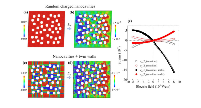
Lu G, Li S, Ding X, et al. (2020) Enhanced piezoelectricity in twinned ferroelastics with nanocavities. Phys Rev Mater 4: 074410. https://doi.org/10.1103/PhysRevMaterials.4.074410 doi: 10.1103/PhysRevMaterials.4.074410
|
| [27] |
Neithalan N, Weiss J, Olek J (2006) Characterizing enhanced porosity concrete using electrical impedance to predict acoustic and hysdraulic performance. Cem Concr Res 36: 2074-2085. https://doi.org/10.1016/j.cemconres.2006.09.001 doi: 10.1016/j.cemconres.2006.09.001
|
| [28] |
Vu C-C, Amitrano D, Ple O, et al. (2019) Compressive failure as a critical transition: experimental evidence and mapping onto the universality class of depinning. Phys Rev Lett 122: 015502. https://doi.org/10.1103/PhysRevLett.122.015502 doi: 10.1103/PhysRevLett.122.015502
|
| [29] |
Soto-Parra D, Zhang X, Cao S, et al. (2015) Avalanches in compressed Ti-Ni shape-memory porous alloys: An acoustic emission study. Phys Rev E 91: 060401. https://doi.org/10.1103/PhysRevE.91.060401 doi: 10.1103/PhysRevE.91.060401
|
| [30] |
Chen Y, Ding XD, Fang DQ, et al. (2019) Acoustic emission from porous collapse and moving dislocations in granular Mg-Ho alloys under compression and tension. Sci Rep 9: 1330. https://doi.org/10.1038/s41598-018-37604-5 doi: 10.1038/s41598-018-37604-5
|
| [31] |
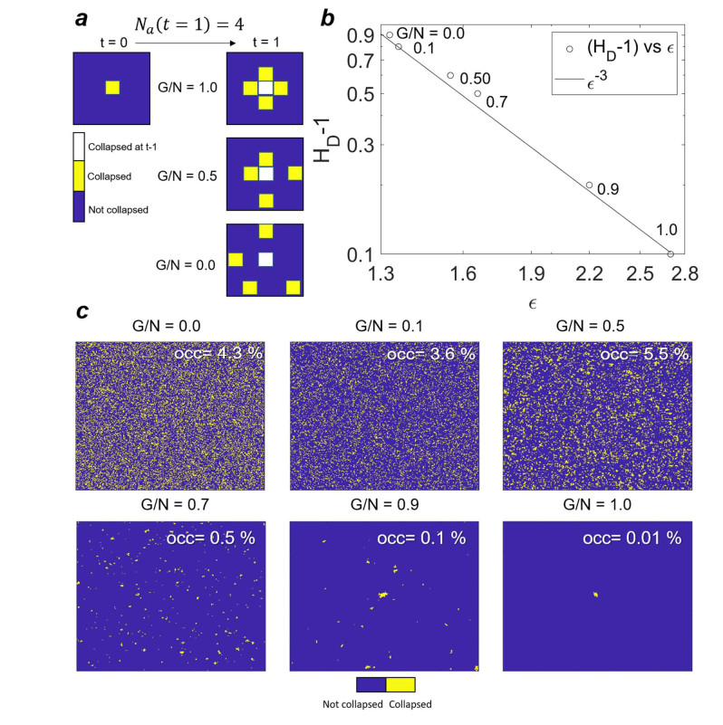
Casals B, Salje EKH (2021) Energy exponents of avalanches and Hausdorff dimensions of collapse patterns. Phys Rev E 104: 054138. https://doi.org/10.1103/PhysRevE.104.054138 doi: 10.1103/PhysRevE.104.054138
|
| [32] |
Bingham NS, Rooke S, Park J, et al. (2021) Experimental realization of the 1D random field Ising model. Phys Rev Lett 127: 207203. https://doi.org/10.1103/PhysRevLett.127.207203 doi: 10.1103/PhysRevLett.127.207203
|
| [33] |
He X, Ding X, Sun J, et al. (2016) Parabolic temporal profiles of non-spanning avalanches and their importance for ferroic switching. Appl Phys Lett 108: 072904. https://doi.org/10.1063/1.4942387 doi: 10.1063/1.4942387
|
| [34] | McFaul LW, Wright WJ, Sickle J, et al. (2019) Force oscillations distort avalanche shapes. Mater Res Lett 7 496-502. https://doi.org/10.1080/21663831.2019.1659437 |
| [35] |
Casals B, Dahmen KA, Gou B, et al. (2021) The duration-energy-size enigma for acoustic emission. Sci Rep 11: 5590. https://doi.org/10.1038/s41598-021-84688-7 doi: 10.1038/s41598-021-84688-7
|
Figures(3)

Ekhard K.H. Salje. Porosity in minerals[J]. AIMS Materials Science, 2022, 9(1): 1-8. doi: 10.3934/matersci.2022001


 DownLoad: