The least squares Bisymmetric solution of quaternion matrix equation $AXB = C$

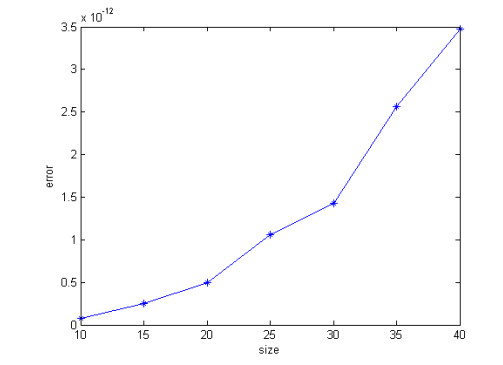
1.   Introduction and motivations

In this work, we focus on developing a best mathematical approach for the so-called systematic risk or capital asset pricing model using wavelet theory. Recall that such a theory has been proved to be a powerful tool in the economic/financial field. Financial indicators are subject to volatility and high fluctuations in all markets, which makes their study and their understanding using classical methods un-sufficient. One of the main power characteristic of wavelets is their ability to detect and/or localize fluctuations and volatility.

Financial markets are the essential component of countries' economies. All industrial countries have at least one purse and most developing countries have created one or have to create. Financial markets have enabled economic agents to reconcile the antagonistic objectives of their clientele. These are objectives of profitability, security and liquidity. To obtain portfolios that combine high levels of profitability with high levels of security and thus being less risky, financial market participants have several financial asset management instruments. Earlier, in the 50th of the last century, Markowitz (1952) has put the basics of the theory of financial asset management and the functioning of the financial markets leading to a rigorous link between risk and return on securities. Next, the studies have been growing up in both theory and empirically. See Sharpe (1964), Lintner (1965a), Lintner (1965b), Mossin (1966) and Black (1972), Black et al. (1972). Henceforth, the CAPM become a central model in financial theory that makes it possible to describe in a simple way the link of profitability of financial assets and their risks. The validity of the CAPM has been by the next investigated by Roll (1977) based on USA market and stating that the omission of some low capitalization securities could affect the CAPM. In addition, all assets such as bonds, gold and real estate should be taken into account.

More recently, the CAPM has been improved by several empirical studies. In particular, Fama and French (1996) announced the death of systematic risk beta, using annual data of the well known indexes NYSE, AMEX, and NASDAQ returns during the period time 1963 to 1990. They stated that the systematic risk beta may not provide a strong indication for explaining the average change in the market index. Re-considered next by Kothari and Shanken (1998), results of Fama and French (1993) have been proved to be more significant by using monthly data on equity returns rather than annual data. Even though, Kothari and Shanken (1998) noticed that the use of annual returns to estimate the beta may be a cause of measurement problems. This is essentially due to the seasonal effect of returns, the non-synchronization of actions, etc. Based on the annual returns from 1927 to 1990, the authors concluded that the beta is statistically significant and that the regular contribution of size to explain the difference in sample yielded beyond the beta is minimal. For a deep backgrounds on CAPM the readers may refer to Aydogan (1989), Banz (1981), Basu (1977), Black (1972), Black et al. (1972), Breeden (1979), Chae and Yang (2008), Chan and Lakonishok (1993), Fama and MacBeth (1973), Fama and French (2004), Fama and French (2006), Galagedera (2007), Gibbons (1982), Gursoy and Rejepova (2007), Handa et al. (1989), Handa et al. (1993), Ho et al. (2000), Karan and Karadagli (2001), Merton (1973), Perold (2004).

Some empirical extensions of the CAPM taking into account the time variations of beta and time variations of the risk premium or both of them have been developed. The so-called CAPM Conditional Testing has been established joining an old study on the same subject due to Levhari and Levy (1977) where the use of a shorter time than real time has been proved to provide biased beta estimator. Handa et al. (1993) showed that if the difference in the time interval of the returns is taken into account, for the same action, different estimators can be obtained. Furthermore, Handa et al. (1993) rejected the beta estimator that uses monthly returns and accepted instead the use of annual returns. Cohen et al. (1986) showed that the beta estimator is sensitive to the time intervals used for equity returns. As a result, the problem of the validity of the CAPM arises, and more particularly the validity of the relationship between the systematic risk and the return of securities listed on the financial markets taking into account the time factor in the returns of the shares. This key issue of the CAPM audit, which has already been the subject of extensive research in industrialized countries, is still relevant.

As mentioned by Marfatia (2017a) and Marfatia (2017b), one of the limitations of conventional approach is the lack of distinction between the time domain and the frequency ones which is a crucial task in both econometric and economic rationale.

The present study lies in the whole scope of the integration and/or the study and evaluation of risks in stock markets according to time changes. Many studies have been developed to do such task. In Marfatia (2017a) a wavelet-based study has been developed to investigate the impact of risks in international stock markets. The approach proposed in Marfatia (2017a) consists in combining wavelet techniques with time-varying conditional volatility to investigate essentially the co-movement of risks at both the country level and regional level. The authors concluded that co-movement of risks between the US market and European markets are strong mostly at lower frequencies. However, the co-movement of risks between the country and its local region are strong at higher frequencies. Moreover, at high frequencies the relationship between the country in hand and the US or other global markets is also weak. The study concluded also that the spill-over of risks are mostly limited at lower frequencies contrarily to existing studies which claim that especially during the recent financial crisis, the spill-over of risks are largely a global phenomenon.

In Marfatia (2017b), linkages of the housing market and macroeconomy has been investigated using wavelet approach. Cross-wavelet coherence has shown that the relationship varies significantly relatively to countries, time, frequencies, and the direction of causation. The author claimed that house price movements are related to interest rates at short-run, however per capita income growth is related to the interest rates at the long-run. Moreover, the author studied the role of industrial production and income growth and concluded that the direction of causation between the housing market and macroeconomic variables depends strongly on time-frequency domain.

Our main aim here is to understand the nature of the relationship linking systematic risk and the return on equities for GCC stock markets by using wavelet theory as a mathematical tool recently introduced in the field of finance and proved its performance compared to classical tools. A new method to forecast systematic risk based on wavelets for missing data and further exploring the relationship between the return of the stock and its systematic risk at different time scales is proposed.

Wavelets offer efficient algorithms for practical problems where classical techniques have shown limitations. Moreover, they provide an attractive mathematical formalism in the reformulation of several problems and in different scientific fields, especially in time series analysis. Wavelets form a mathematical tool that transforms time domain data into different frequency horizons. They represent the advantage of being localized in both the time and frequency domains. They allow to observe and to analyse data at different time scales, which in turns makes it possible to overcome the inadequacies of the classical analysis of the CAPM. For more backgrounds on wavelets and their applications the authors may refer to Arfaoui et al. (2017), Arfaoui et al. (2020), Arfaoui et al. (2020), Mabrouk et al. (2008), Mabrouk et al. (2008), Mabrouk et al. (2010), Mabrouk et al. (2011), Mabrouk and Zaafrane (2013), Mabrouk et al. (2015), Mahmoud et al. (2016), Percival and Walden (2000), Selcuk (2005), Zemni et al. (2019a), Zemni et al. (2019a).

From an empirical point of view, we aim to apply the wavelet technique to estimate the systematic risk of an action relatively to the market return. This validity could also be a real foundation for effective financial decisions. Indeed, the effectiveness of a financial decision depends to a large extent on the accuracy of the valuation of the securities as well as the most precise knowledge possible of their subsequent evolutions and their risks. We therefore try, in this work to provide a better comprehension of the GCC financial markets in the face of a modern financial theory such as the CAPM.

To resume, one aim in the present research is to find a mathematical approach to the GCC market indices by applying wavelet methods. The new idea consists in applying random and/or different time supports allowing the subdivision of the whole support into random parts instead of using the classical sampling (weeks, months, years). We recall in particular, that the Kingdom of Saudi Arabia has established 2030 projects that have a direct impact on the national market as well as the rest of the Arab Gulf and international markets such as and particularly NEOM project which will have a profound impact on the market. This makes it of interest to study such market and understand its complexities.

The proposed procedure is acted on samples composed of stocks in GCC markets actively traded over a critic period strongly and directly related to the last political changes especially in Arab countries, the GCC embargo against Qatar country. The period may also be considered as a pre-corona stage as we now see that the current pandemic COVID-19 has been spread in quietly all the world. GCC continent is one of the places that are related to all the world because of their geographical position and their strong relation to the worldwide economies as biggest petroleum countries. Moreover, the largest workers community is focusing in these countries. Saudi Arabia is also characterized by the saint cities of Muslims which consequently bring a big number of pilgrims and visitors each year. This may be a strong cause of dispersion of viruses which may be next transferred with pilgrims to other continents. Saudi Arabia has also made a worldwide program known as NEOM international project which is the basic point in the 2030-vision of the kingdom. The sample of study will be based on Tadawul index during the period from January 01, 2013 to September 20, 2018. Notice that this period is also characterized by the direct link to Syrian and Yemen movements and the present Arab war against some parties in Yemen which is somehow leaded by Saudi Arabia. We will discuss the effect of such links on the stability of GCC markets. We may also recall many financial movements such as Aramco subscription and generally the 2030 KSA vision. The findings in the present work may be a good basis for understanding GCC markets situation, behavior and future and thus a basis for investors' decisions in such markets.

We recall that in the data basis applied, the main problem confronted is the lack of data where the samples present missing values for many cases. Consequently, our work becomes a twofold study. In a first step, we developed a wavelet-based method to reconstruct missing data which by the next leads to complete and adjusted basis on the whole period above. The complete basis is applied next for CAPM and thus the comprehension of the Saudi Tadawul market.

The rest of the present work is organized as follows. In section 3, a literature review on forecasting systematics risk is briefly presented. Section 4 is devoted to the development of our methodology. We especially re-develop the wavelet analysis of time series briefly to apply it by the next for missing data reconstruction which in turns will be applied for completing the data basis used later. The mathematical formulation of the CAPM is provided by the next. Finally, this section is achieved by the development of the wavelet CAPM. Section 5 is subject of our empirical results and their discussions on the KSA Tadawul stock market. Section 6 is a conclusion. Finally, section 7 is an appendix in which we provided empirical results of the 3-scale law as a supplementary part to section 5 to improve the idea of time changes in stock market prediction.

2.   Systematic risk forecasting literature review

We propose in this section to conduct a literature review on the systematic risk forecasting. However, we will not be addressing mathematical formulations in this section and include them instead in the methodology section to provide readers a more comprehensible mathematical methodology.

The CAPM was firstly discovered by Sharpe (1964) and next Lintner (1965a), Lintner (1965b). It has been applied next for half a century in estimating the capital cost for companies and evaluating the performance of managed portfolios. However, its empirical evaluation has been always affected by the availability or not of the data. The empirical problems of the CAPM might reflect theoretical failures arising from many superficial assumptions.

The CAPM is based indeed on several assumptions, such as mono-periodicity, the market perfection aspect without taxes nor transaction costs, homogeneity in anticipations, unlimited short selling, loans and borrowing at the risk-free and limitless rate, strictly increasing and strictly concave Von-NeumannMorgenstern utility functions, mean-variance preferences based on restrictions relating to the return or the utility function, investor aversion to risk, competition and market efficiency. However, such assumptions might not be generally accepted simultaneously, which yields limitations for the CAPM. As a consequence, some solutions have been proposed such as the CAPM with taxes (Brennan (1973), Litzenberger and Ramaswamy (1979)), the CAPM with transaction costs (Lévy (1978)), the CAPM in continuous time (Merton (1973)) and the CAPM with non-homogeneous anticipations (Sharpe (1970a), Sharpe (1970c), Sharpe (1970b)).

The choice of a portfolio is generally made after a financial analysis of a set of more or less independent actions. Robust measurement of the crucial variables in the investment decision should be ensured. Numerous studies have investigated the financial analysis of individual actions allowing to make a good decision. Markowitz (1952) has shown that the investor seeks to optimize his choices by taking into account the expected return on his investments and the risk of his portfolio. His model suggests selecting several stocks based on statistical criteria such as the profitability of a stock in order to obtain optimal portfolios. However, Vasichek et al. (1972) asserted that the profitability of a stock is not sufficient to characterize an investment opportunity. The dispersion of returns around the average return reflects the uncertainty of the investment (the risk). The total risk of a portfolio can always be measured by the variance or the standard deviation of its profitability which constitutes a convenient measure of dispersion. This allows investors to minimize the risk of their actions.

According to Markowitz, the CAPM is used to solve the problem of the portfolio structure which incorporates the quantified treatment of risk by estimating the demand function of assets. This makes it possible to study the equilibrium of the market. Such a method has a main drawback as it does not take into consideration the time factor, which causes a strong limitation.

The CAPM is a diagram that analyses the return and risk of an investment. Sharpe (1964) and Lintner (1965b) suggested to estimate the prices of transferable securities allowing supply and demand to be balanced and allowing a general equilibrium of the market. Therefore, the CAPM can determine the prices of equilibrium securities through supply and demand according to a linear relationship between portfolio profitability and total risk. Indeed, the level of risk is obtained by varying the loan or the borrowing which can be made up of all the securities listed on a market. Thus, any combination of an equity portfolio and an investment in the risk-free asset will be indicated by a straight line in the risk-return space. Therefore, any portfolio, by definition, is perfectly diversified, since it involves all stocks in the proposals of their market capitalizations.

Mathematically, for a market in equilibrium, for any portfolio or asset, the CAPM is expressed by means of a linear relationship between the expected return on the share or portfolio $i$ and the market premium where the linearity coefficient is often denoted $\beta_i$ and is known as systematic risk or beta. This coefficient is mainly used for two purposes. The first involves the ranking of assets and portfolios against systematic risks by practitioners. The second aims to test the mean-variance efficiency. Beta is usually estimated using the standard market model, which is expressed by the linear regression model. It also represents the coefficient of elasticity of the price of the security with respect to the stock index representing the market.

Sharpe (1964) proved that for each share i relating to a given portfolio the systematic risk $\beta_i$ is expressed by the quotient of the covariance between the rate of return of asset $i$ and the rate of return of the portfolio by the square of market risk. More precisely, the expected return on security $i$ is expressed by the risk-free interest rate increased by a risk premium composed of two elements. The first element is the excess of the expected market rate of return over the return on the risk-free asset, measuring the risk premium that the investor should perceive by agreeing to bear a risk equal to that of the market. The second element $\beta_i$ is the measure of the importance of the risk of security $i$ in relation to the risk of the market. Sharpe (1970b) and Vasichek et al. (1972) concluded firstly that the CAPM is purely normative, subject to empirical validation and secondly that the rate of return of each share in excess of the risk-free interest rate depends only on $\beta_i$.

The CAPM gives a coherent answer, as for the evaluation of the expected profitability of an asset according to the risk. This profitability can be used as the discount rate in the valuation of the asset. Indeed, the relationship between the risk and the profitability of a financial asset is linear, provided that this risk is measured by its variance with the market taken as a whole and not its variance or its standard deviation. Each investor has the choice between obtaining a certain but low profitability or taking a risk offset by a higher expected profitability. Markowitz was the first to formalize and quantify the diversification effect according to which a combination of many assets in a portfolio reduces the total risk for a given expected rate of return.

Sharpe W. F. considered a model which results in the equilibrium relationship between the expected profitability of a financial asset and its risk. This model makes it possible to determine the choice of investment and to compare alternatives to different random gains by using the Esperance-Variance criterion in order to choose the best alternative.

In the same context, Von Neuman and Morgestern in the 1944-th formally proved that any individual yielding to a few intuitive axioms of rationality aims to maximize the expectation of the utility of their wealth. Indeed, the utility function reflects the preference of each individual, hence each individual is specific, and depends in particular on his initial wealth at the time of the decision and his aversion to risk. The conclusion lies in the fact that the individual faced with alternatives with random consequences aims to maximize the expectation of utility.

Diversification is also an important factor in estimating the CAPM. It is strongly related to the behaviour of the expectation-variance of the portfolio. The profitability of the portfolio is the weighted average of the expectations. The contribution of each security to the expected profitability of the portfolio is therefore proportional to its expected profitability. In terms of risk, it is possible to measure that of the portfolio by the variance of its profitability.

According to Markowitz, an efficient portfolio is characterized by a maximum expectation of return or by a minimum variance for a given expectation of return. The efficient frontier is the set of all efficient portfolios. The efficient frontier takes two different forms depending on the absence or presence of a risk-free return asset. The minimum variance frontier determines portfolios of risky assets and shows the lowest risk for a given level of profitability. As for the portfolios with the highest levels of profitability for a given level of risk, they are represented by the efficient frontier corresponding to the upper part of the frontier at minimum variance.

However, several criticisms have been pointed out for the CAPM (Desmoulins-Lebeault (2003), Magni (2007a), Magni (2007b)). Some are linked to the portfolio and some are linked to market. Roll (1977) introduced an empirical criticism due to the representative portfolio of the market. This portfolio groups together assets held by a set of investments, a set of stocks, bonds and other types of securities that are not in practice negotiable and liquid such as real estate assets of investments and their human capital. This puts into question the results of the econometric tests and the practical utility in terms of management and performance analysis. Roll (1977) claimed that according to CAPM, the ideal portfolio is able to positively manage the different variables. Roll (1977) discussed the problem of the right of the market. It is a conceptual order that challenges the theoretical foundations of investment performance indicators over another period of time. If the market portfolio is efficient, securities are on average to the right of the market. It is therefore sometimes impossible to observe deviations from this line over a long period. In reality, these deviations do not indicate whether a security is over or under-priced.

The estimated betas are relative for the entire period studied and assumed to be stable relatively to a certain scale. While in reality the variance with the market varies over time and therefore there may be some statistical issues related to errors in the beta estimates of individual securities and their instabilities which are not taken into account.

Overall, the CAPM formulation showed remarkable empirical robustness in determining excess return, taking systematic risk into account. CAPM is characterized by a special case which forms several types of risk into one defined by systematic risk (non-diversifiable risk or market risk). In this sense, two securities with the same level of risk can lead to different profits. Investors tend to choose the security with the highest profit. This choice will lead to a drop in profit. However, if there are two portfolios A and B of the same risk, where B is the optimal portfolio according to the CAPM, portfolio A generates a higher return than that of B. In such a case, investors who seek new opportunities will be willing to invest in A although it is undervalued by the CAPM, and to sell the optimal portfolio B which has the same systematic risk.

Besides, other studies have focused on empirical extensions of the CAPM taking into account the time variations of the risk beta or variations in the time of the risk premium or both of them. This area of research is often referred to as the CAPM conditional test. Studies on this topic show the major impact of time intervals on the estimate of beta, understanding of the market and the economic policies in general (See for instance Levhari and Levy (1977), Marfatia (2014), Marfatia (2015), Marfatia (2017a), Marfatia (2017b), Marfatia (2020)). Handa et al. (1993) showed that if the difference in the time interval of returns is taken into account, for the same action, we may obtain different estimators. Handa et al. (1993) rejected the CAPM beta estimator which uses monthly returns, but accepted the one based on annual returns. Cohen et al. (1986) showed that the beta estimator is sensitive to the time intervals used for stock returns.

Consequently, the problem of the validity of the CAPM according to time variation arises. More precisely, the validity of the relation between the systematic risk and the return of the securities quoted on the financial markets taking into account the time factor in the returns of the equities seems to be necessary. This essential issue of CAPM verification is still relevant today. To our knowledge, few works have looked specifically at this question, in particular by using a method as powerful as that of wavelets. The time-scale division induced by the wavelet transform overcomes the shortcomings of the classical CAPM analysis.

Our objective here is to test the validity of the CAPM on the Saudi Arabia Tadawul market. We aim firstly to analyze the systematic risk and to point out its limitations taking into account the time factor. The second is to identify the relationship between equity returns and their systematic risks in the Saudi Arabia Tadawul market using the wavelet approach taking already the time factor into account.

In our knowledge, the application of wavelets for GCC stock markets is still recent and the literature on it needs more developments. However, in other markets such a tool is now developed and has induced more understanding for the markets analyzed such as SP500 (USA), CAC40 (France) and ISE (Istanbul). Gençay et al. (2003) applied wavelets for the stock markets of the US, UK and Germany to estimate the best time scale for measuring systemic risk. The authors concluded that the relationship between risk and return is a multi-scale phenomenon. Fernandez (2006) analyzed the Santiago stock market in Chile using time-scaling methodology. Rhaiem et al. (2007a), Rhaiem et al. (2007b) studied the French CAC40 index as market portfolio and the daily EURIBOR as the risk-free rate. The predictions of the CAPM are claimed to be more relevant in the short term than in the long term, which makes the French market different from those of the US, UK and Germany. Aktan et al. (2009) applied the wavelet multi-scaling method for the Istanbul Stock Exchange during the period from January 2003 to October 2007. It is shown that a positive relationship between risk and returns is most significant at the medium levels, concluding that the effect of market returns on an asset is stronger in this time horizon.

3.   Methodology

Before introducing the methodology applied in our work it is necessary to recall some basic facts. Indeed, one of the important factors that may affect the model described here may be the US policy actions and the risk perceptions which significantly impact international stock markets. However, we did not include these factors in the present model as our aim is not to change the CAPM model which already exists but to improve it firstly by using the wavelet time-frequency action. This fact may be considered as a limitation for the present work and opens instead a good idea for an eventual extension. Besides, some recent studies have discussed the role of these factors and their estimations in other models which confirms their importance and the motivation to include them in any eventual extension of the present model. Indeed, in Kishor and Marfatia (2013) time-varying response of foreign stock markets to US monetary policy shocks has been estimated. The authors noticed a significant time-variation in the response of the global equity markets to US monetary policy surprises especially during the crisis periods. The model applied looks like the present one as it aims to estimate a risk-like parameter $\beta^i$ as follows

where $R_t^i$ is the abnormal return of country $i$ at the event date $t$ and $\Delta r_t^u$ is the monetary policy surprise. The coefficient $\beta^i$ reflects the response of the abnormal return of a country $i$'s stock market to unanticipated interest rate increase in the US.

Now our methodology consists in a first step to apply wavelet decomposition of time series to overcome the problem of missing data confronted when gathering the data applied in our work. Next, as the data is completed the whole basis will be subject of both CAPM and wavelet CAPM processing.

3.1.   Wavelets for time series

Wavelet analysis allows the representation of time series into species relative to the time and frequency information known as time-frequency decomposition. It consists in decomposing a series in different frequency components with a scale adapted resolution and thus permits to observe and to analyze data at different scales. Wavelet analysis starts from one source function $\psi$ known as the mother wavelet and next composes dilation-translation copies to get a complete system for finite energy time series. Each wavelet basis element is defined for $j, k\in\mathbb{Z}$ as a copy of $\psi$ at the scale $j$ and the position $k$ by $\psi_{j, k}(t) = 2^{-j/2}\psi(2^jt-k)$. The quantity $2^j$ corresponds to the frequency of the series while the index $k$ localizes volatility or fluctuations. Let for $j\in\mathbb{Z}$ fixed, $W_j = span(\psi_{j, k}, \, k)$ known as the $j$-level detail space. A time series $X(t)$ is projected onto $W_j$ yielding a component $DX_j (t)$ given by

The $d_{j, k}$ are the detail coefficients of the series $X(t)$ expressed by means of the ordinary inner product in the functional space $L^2(\mathbb{R})$ as

The spaces $W_j$'s form an orthogonal decomposition covering the space of finite energy series $L^2(\mathbb{R})$. This means that the series $X(t)$ can be completely reconstructed as a sum of its projections on the detail spaces and that these projections are mutually uncorrelated. In wavelet theory, the mother wavelet yields a second function called father wavelet or scaling function denoted here by $\varphi$. (See Daubechies (1992)). Similarly to $\psi$, the function $\varphi$ yields dilation-translation copies $\varphi_{j, k}(t) = 2^{-j/2}\varphi(2^jt-k)$ generating subspaces $V_j$. The sequence $(V_j)_j$ is called a multi-resolution analysis (multi-scale analysis) on $\mathbb{R}$ and $V_j$ is called the $j$-level approximation space. It is well known in wavelet theory that $V_j\subset V_{j+1}$, $j\in\mathbb{Z}$, which means that the approximation of the time series at the level $j$ and $j+1$ can be viewed from each other and so from any horizon $p\geq j+1$. In physics-mathematics this is called the zooming rule. It holds also that for all $j\in\mathbb{Z}$, $f(t)\in V_j$ iff $f(2t)\in V_{j+1}$, which reflects the fact that, not only the signal $f$ from horizon $j$ can be seen in the horizon $j+1$ but also his contracted or dilated copies. As for the detail subspaces, the approximation subspaces $V_j$'s satisfy also a completeness relation meaning that no information is lost when considering all approximations and a second property meaning that all the information is lost at finer scales. Finally the $Vj$'s satisfy a shift-invariance property in the sense that $f(t)\in V_j$ iff $f(t-k)\in V_j$, $j, k\in\mathbb{Z}$, which means that the multi-resolution analysis permits to detect the properties of the signal along the whole time support. Combining all the properties above we deduce that the approximation space is decomposed into a low-level approximation part supplemented with a detail one. Under these properties, the following decomposition is proved for $j\in\mathbb{Z}$,

The component $AX_J(t) = \sum\limits_{j\leq J}DX_j(t)$ is called the approximation of $X(t)$ at the level $J$ and it reflects the trend or the global shape of $X(t)$. It also belongs to the space $V_J$. Thus, using the definition of the $V_J$'s, the component $AX_J (t)$ may be expressed using the basis $(\varphi_{J, k})_k$ as

where the $a_{J, k}$ are the approximation coefficients of the series $X(t)$ expressed by $a_{J, k} = < X, \varphi_{J, k} >$. As a result, we obtain the following relation known as the wavelet decomposition of $X(t)$

It is composed of one part reflecting the global behavior of the series and a second part reflecting the higher frequency oscillations or the fine scale deviations of the series near its trend. In practice we cannot obviously compute the complete set of coefficients. We thus fix a maximal level of decomposition $J$ and consider the decomposition for any $J_0 < J$,

There is no theoretical method for the exact choice of the parameters $J_0$ and $J$. However, the minimal parameter $J_0$ does not have an important effect on the total decomposition and usually chosen to be 0. But, the choice of $J$ is always critical. One selects $J$ related to the error estimates.

In finance, economics, management and generally actuarial sciences, compared to classical theories wavelet analysis is still less used although it proved good results and needs to be more developed. Recently the literature starts growing rapidly. See Arfaoui et al. (2017), Arfaoui et al. (2020), Arfaoui et al. (2020), Mabrouk et al. (2008), Mabrouk et al. (2008), Mabrouk et al. (2010), Mabrouk et al. (2011), Mabrouk and Zaafrane (2013), Mabrouk et al. (2015), Conlon et al. (2008), Cifter and Ozun (2007), Cifter and Ozun (2008), DiSario et al. (2008), Fernandez (2006), Gençay et al. (2002), Gençay et al. (2003), Gençay et al. (2005), Mahmoud et al. (2016), In and Kim (2006), In and Kim (2007), In et al. (2008), Percival and Walden (2000), Selcuk (2005), Sharkasi et al. (2006), Xiong et al. (2005), Yamada (2005), Zemni et al. (2019a), Zemni et al. (2019a).

3.2.   Wavelets for missing data in markets

As mentioned in the introduction, the main problem in studying markets' movements and/or situations is the lack of data and sometimes its uncertainty. This leads researchers to develop prior procedures to complete the data used in the market study. In our situation here this problem is present strongly in the data used. We noticed that the origin of our data results in some missing values in many actions shared in the market index used here and which is the well-known Tadawul index of the Saudi stock market. To overcome this problem and instead of searching left and right for the data and confronting may be with the same problem in other origins, we proposed to act a wavelet method to reconstruct missing values. The data basis is essentially extracted from the web site www.investing.com

The present section is devoted to present the wavelet-based method to reconstruct such missing data. The method consists in providing a prediction procedure able to predict a short time interval series on an arbitrarily set of backwards and/or forwards (past and/or future, prior and/or post) values. Recall that generally to conduct a best prediction or reconstruction of time series we need usually a long-time interval for training. This fact may not be satisfied in general situations. For some situations such as ownership-structure and diversification variable the samples are usually short. One has one main value on a year. Furthermore, when applying wavelet analysis to approximate and/or to forecast time series, the majority of the existing studies assume the presence of some seasonality, periodicity and/or autoregressive aspect in the series. See for example Mabrouk et al. (2010), Soltani (2002), Soltani et al. (2007) and the references therein.

In the present paper, we act a simple method already tested in Mabrouk et al. (2010) leading to good prediction. The method is principally characterized by the non-necessity to test it on the detail parts components of the series nor its wavelet coefficients. This is essentially due to the fact that we use few values of series leading to short sub-samples and next act the prediction on the sub-samples. In such parts the dynamic behavior is not important. However, the most positive point in the method is the fact that it necessitates only to compute the values of the source scaling function and the associated wavelet on a suitable grid, the dyadic or the integer grid in the supports of the mother and father wavelets.

Let $X(t), \, t = 1, 2, \dots, N$, be a time series. The procedure to be applied is a dynamic recursive scheme consisting in applying firstly a partial estimator at short horizons to all the observations $(t_i, X_i), \, i = 1, 2, \dots, N$, to yield firstly the predicted value of $X_{N+1}$. This last is then included as new observation to predict $X_{N+2}$. We then follow the same steps until reaching the desired horizon. During the procedure, we apply the $J$-level wavelet decomposition (4). This necessitates to know the values of the mother wavelet $\psi$ on the dyadic grid $\{2^j(N+1)-k, \, k\}$ and the scaling function $\varphi$ on the integer grid $\{N+1-k, \, k\}$ in the supports. Assume we have got $X_J(N)$. The next value will be estimated by ($J_0 = 0$ in (7))

This means that for evaluating the predicted value of $X_{N+1}$, it suffices to do this for $AX_J$ and the $DX_j$'s. This motivates the use of Daubechies compactly supported wavelets which are well evaluated on the integer grid.

3.3.   The mathematical formulation of the CAPM

The selection of a portfolio is usually preceded by a financial analysis of a set of stocks. A good analysis provided with a successful quantification of the important variables of the investment decision on the financial markets will be a central factor for investors success. One of the variables is the profitability, defined as the sum of capital gains and dividends reported at the beginning of the period. The expected profitability of a portfolio is equal to the weighted average of the expected returns on the different securities that make it up. A second factor is the risk of an action. Recall that the dispersion of returns near the average profitability reflects the uncertainty or the risk of the investment. The standard deviation and/or the variance are convenient measures of this dispersion. To avoid risk, investors prefer investing with a low variance.

In its original and/or simple variant, the CAPM is mathematically expressed as

where $R_{i, t}$ is the return rate of an action $i$ at the period time $t$, $R_{m, t}$ is the return of the market measured by means of a general index at the same period of time $t$. The parameter $\beta_i$ is a specific factor to each action $i$, indicating the relation between the fluctuations of the action $i$ return rate and the fluctuations of the general index of the market, called often the beta coefficient or the systematic risk. The factor $u_{i, t}$ is a random factor representing the hidden fluctuations of $R_{i, t}$ that are not explained by the market, or generally an error term. Finally, the parameter $\alpha_i$ is added to guarantee a null expectation of $u_{i, t}$. Therefore, CAPM breaks down the total variability of an action into two parts. A first part, due to the influence of the market and which corresponds to the systematic risk and a second due to the specific characteristics of the action and which corresponds to the variations of the specific prices of such action, called sometimes the diversified or the specific risk. The CAPM allows to study the behavior of all operators in a market and to build a theory of equilibrium. The market is a global reference framework defining the conditions that prevail in all the transactions that economic agents carry out. It allows the confrontation of supply and demand. The equilibrium is reached under many hypotheses such as the null transaction cost, the perfect divisibility of assets, free-tax dividends, and capital gains, intervention of both buyers and sellers in the market without influencing prices. We may also consider the possibility that investors can lend or borrow required amount at a pure interest rate, without influencing the level, and the borrowing rate is equal to the loan rate. Some hypothesis are also based on investors behavior such as risk aversion behavior, equality of expectations for operators as to profitability expectations associated with the different assets and their risks, the rationality and safety of operators over a given horizon, to maximize their wealth.

Many variants of the mathematical CAPM formulation have been developed in the literature. Sharpe (1964) proposed a variant of CAPM based on expected returns stating that

which by setting $\beta_i = \dfrac{\sigma_{im}}{\sigma_m^2}$ becomes

It means that the expected return of the action $i$ is estimated by the risk-free interest added with a risk prime. This later is composed of the excess of the expected rate of return of the market minus the remuneration of the risk-free asset multiplied by the factor $\beta_i$. It thus depends on the risk premium that the investor should receive when agreeing to bear a risk equal to that of the market and the importance of the risk of the action $i$ against the risk of the market. In literature, there are other categories of the CAPM such that CAPM without a risk-free asset and CAPM with transaction costs. See for example Black (1972), Black et al. (1972). Assume that a number $K$ of investors are present. The $k$-th investor will allocate his wealth $T_k$ in a number $M_k$ of actions in the market. To be in an equilibrium situation, we should have

where $E_i$ is the expectation of the return of action $i$, $E_k$ is the expectation of the return of the optimal portfolio detained by the investor, $\sigma_k^2$ is the variance of the optimal portfolio and $\sigma_{ik}$ is the covariance between the return of action $i$ and the portfolio. Denoting similarly to previous variants $\beta_{ik} = \frac{\sigma_{ik}}{\sigma_k^2}$ the last equation becomes

$\beta_{ik}$ is the volatility of the action $i$ relatively to the optimal portfolio. Taking into account all investors wealth, Lévy (1978) proposed the form

where $TK = \sum\limits_{k = 1}^{K}T_k$. This formula means that the required risk premium of the action $i$ is evaluated as the average of the premiums demanded by the investors, weighted by their respective wealth.

CAPM may also depend on inflation. Indeed, assuming the existence of an asset with certain nominal return, Friend et al. (1976) proposed that the relation between the risk and the return of the different assets could be written as

where $\sigma_{i\pi}$ is the covariance between the rate of return on assets $i$ and the rate of inflation, $\sigma_{m\pi}$ is the covariance between the market rate of return and the rate of inflation and $\alpha$ is the ratio between the nominal value of risky assets and that of all assets.

Finally, taking into account the taxation, the CAPM may be modified to reflect the presence of taxation based on the relationship between the expected return and the risk of the security as

where $E_i$ is the expectation of the yield of action $i$, $T_0$ is the tax rate, $\beta_i$ is the systematic risk and $E_m$ corresponds to the expectation of the market return.

Different forms of the CAPM may be also found in the literature that take into account other factors such as heterogeneity of anticipations relatively to future performances of actions, etc. See for example Aktan et al. (2009). In the present paper, we assume that the CAPM defines the required return on an investment according to the equation

where $E(R_i)$ is the asset's expected return, $r_f$ is the risk-free rate, $E(R_m)$ is the expected return of the market portfolio, and $\beta_i$ is the measure of risk for asset $i$ evaluated as

In empirical finance, $\beta_i$ is estimated usually via the ordinary least square estimate from the linear regression

where $\varepsilon_{it}$ is the error term while $\alpha_{it}$ is a constant. Consequently, the risk beta allows to decompose the variance of an asset $i$ as

Hence, the variance $\sigma_i^2$ can be decomposed into a first component $\beta_i^2\sigma_m^2$ corresponding to the firm's systematic risk and a second one $\sigma_{\varepsilon_{i}}^2$ corresponding to the firm's unsystematic risk.

3.4.   The wavelet CAPM

To estimate the CAPM with wavelets the first step is to pass by the variance and the covariance of the statistics (time) series and introduce the analogues for the components due to the wavelet decomposition. Therefore, the wavelet analysis consists here also in splitting the variance of the series into sub-variances relative to scales or the levels $j$ which will be called the variance of the series at the scale $j$ (Percival and Walden (2000)). Let $\upsilon_X^2$ be the variance of $X(t)$ and $\upsilon_X^2(j)$ be the variance of the projection at the scale or the level $j$, we have

This permits to focus on the sub-variances of the components at a level j instead of considering the whole series. This in turns facilities the analysis of the fluctuations and the dynamics of the series. Denote $L$ the length of the wavelet support, $N_j = [N/2^j]$ the number of wavelet coefficients at the level $j$ and $L_j = [2^{-j}(L-2)(2^j-1)]$ the number of boundary wavelet coefficients at the level $j$. The variance at the level $j$ is estimated as

Similarly, we have an analogue formulation for the covariance at the level $j$ for a couple of series $(X, Y)$ as

To apply wavelets for evaluating the CAPM we firstly decompose returns into their wavelet decompositions. This leads to component-wise returns according to the levels. These new time series will be considered as the returns to be applied. See for example Gençay et al. (2003). The risk beta will be estimated by the wavelet risk beta at the level or the scale $j$ as

where $\widehat{\upsilon}_{R_iR_m}(j)$ is the wavelet covariance of the component $i$ of the portfolio with the market at the scale $j$. $\widehat{\upsilon}_{R_m}^2(j)$ is the wavelet variance of the market at the scale $j$.

Next, in order to illustrate the explanatory power of market returns on the determination of portfolio returns, we estimate the coefficient $R_i^2(j)$ for each time scale used as follows

4.   Empirical results and discussions

One of the main facts in analyzing stock markets is the uncertainty phenomenon related to many factors such as data collection and recording, policy makers, etc. In Marfatia (2014) the impact of monetary policy on the real economy has been investigated based on policy makers and market participants. A novel approach has been developed for evidence supporting the Lucas island model predictions. Based on the estimation of the time varying response of the S & P stock returns to monetary policy surprises derived from the high frequency Federal funds futures market, the study concluded that at higher level of uncertainty, the impact of FOMC policy surprise on the time varying S & P returns decreases. Besides, the volatility in the short-term bond market has been shown to offer highest explanatory power in explaining the impact of uncertainty on the effectiveness of Fed's policy surprises. This study interconnects with the present one in the common point of taking into consideration of the uncertain character of financial data. However, in the present work we considered these uncertain values to be part of missing data and thus a post reconstruction step based on wavelet theory has been conducted to fill the gaps of missing and uncertain data. The study of the affects of such missing and/or uncertain data on the risk may be a good eventual future direction. Moreover, taking into consideration the US policy is of great interest in the model as US policy is strongly affecting the one in GCC countries especially KSA and vice-versa. We may recall here the last phenomenon of floating the oil market which affected immediately the US oil market and thus the US policy makers. We have noticed enormous politicians from both republic and democratic parties that strongly criticizing and threatening to change the way of collaboration with KSA despite their strategic relations.

In Marfatia (2015) the role of financial stress and risks in the monetary policy's time-varying impact on the US bond markets has been studied. The author investigated precisely the link between the treasury and monetary policy shocks and the impact of the financial market volatility. Besides the author concluded that a time-varying coefficient is more adequate to express the impact of the monetary policy on the market and to express adequately the uncertainty in economic data and its role in estimating interest rates as well as the level of financial risks. These facts join in some sense the present work as we suggest here also that time variation is an essential character in estimating the coefficient of correlation between the whole market index and the firms and did not assume that such coefficient remains constant over time. However, our present model did not include neither the US monetary policy nor the GCC monetary policy as explicit factors, despite their importance and their hidden role and hidden affect on the market studied. These factors, which constitute some limitations of the present model, may be interesting extending studies in the future for both the theoretical mathematical model and the decision makers in the market as well as policy makers.

The main object of our work is to examine the effect of time scales on the systematics risk of the stock components of the market. We test the following hypotheses:

● Hypothesis 0: The risk beta is stable according to time scales.

● Hypothesis 1: There is a linear dependence between action's returns and their systematic risks.

This paper empirically tests a wavelet methodology of beta estimation proposed previously on daily data for GCC markets collected on the period of January 01, 2013 to September 20, 2018 resulting of a sample size $N = 1427$ due to the well-known Tadawul index for Saudi Arabia stock market. We focused on a portfolio composed of 148 actions as listed in Table 1 with corresponding sectors. Table 1 provides the components of Tadawul market applied in our study and their classification according to the global classification standards.

In fact, Tadawul stock market is already classified into industrial sectors since 2008. Next, with the continuous developments in KSA economy, new companies as well as industries have emerged into the market. Consequently, necessary changes have been conducted in the classification of companies listed on Tadawul to reflect the emergence of the new elements. However, Tadawul's previous sector classification was not based on global classification standards which induces some limitations in the classification.

In the new Tadawul market structure there are 20 sectors presented as follows: Energy, Materials, Capital Goods, Commercial & Professional Svc, Transportation, Consumer Durables & Apparel, Consumer Services, Media and Entertainment, Retailing, Food & Staples Retailing, Food & Beverages, Health Care Equipment & Svc, Pharma Biotech & Life Science, Banks, Diversified Financials, Insurance, Telecommunication Services, Utilities, REITs, Real Estate Mgmt & Dev't. Table 1 provides the re-organization of the Tadawul stock market components according to the global classification standards reminiscent of a bit modification where we merged some sectors into one according to their closeness. The Consumer Durables & Apparel Components is merged with Consumer Services to constitute the new sector Consumer. The sectors Foods & Bevarage and Food & Staples Retailing are merged to compose the new sector Foods. Finally we merged the sector Health Care Equipment & Svc with the sector Pharma Biotech & Life Science into the new sector Health and Life Science. Consequently we obtain 17 sectors as shown in Table 1, which resembles to the classical segmentation of Saudi market.

The choice of this market is motivated by the fact that Tadawul is the best representative index of the Saudi market supervised by the Capital Market Authority. It is also considered as the largest capital market in the Middle East and North Africa. Recently at the end of 2019, Tadawul has taken place in the first 10 largest stock markets in the world. It lists more than 150 publicly traded companies. We applied in our study a number of 148 ones because of the non-availability of sufficient data and or the very weak effect of some companies in the applied period of study. For example, a first test has yielded for ABIDC action a zero beta for both scale laws of the periods of time applied.

4.1.   Wavelet completion of the data basis

Recall as mentioned in the introduction that when collecting the data about financial GCC markets such as KSA Tadawul applied here, the main problem confronted is the lack of data where the samples present for many cases missing values. Consequently, we started by acting a wavelet method to reconstruct missing data which by the next leads to complete and adjusted basis on the period of study. On the total basis used we noticed 231 missing values dispersed on the whole market and on different time dates (daily) on 14 actions in the market. The complete basis is applied next for CAPM and thus the comprehension of the market. The missing values are distributed as in Table 2. We applied as in Mabrouk et al. (2010) a training set of 5 prior values for different time dates (daily) on 14 actions in the market.

In fact several wavelet functions have been tested to provide a best filtering. The tests results in the well-known Daubechies wavelet Db6. The authors may refer to Daubechies (1992) where a mathematical method has been developed to compute numerically the values of the mother/father wavelet on dyadic points in the compact supports. The essential idea there was based on the fact that the vector of values of the wavelet at these points is an eigenvector for a special matrix associated also to dyadic eigenvalues. In fact, in Mabrouk et al. (2010) we applied a newer version of Daubechies wavelets developed differently and applied also in Mabrouk et al. (2010) based on connection coefficients of wavelets and leading to the fact that the matrices obtained in Daubechies (1992) may be transformed into circulant and hollow ones. This permits a great gain in machine memory, algorithms speed and error estimates.

4.2.   The CAPM processing

Next as our basis of data has been completed to obtain $100\%$ trading days we are able to develop the CAPM analysis. We propose to study the relationship between excess return on each individual stock and the time scales of market portfolio using the usual OLS estimator for $\beta_i$ issued from the regression (19). The daily return of each stock is calculated as the log-price difference

where $P_{i, t}$ is the price of asset $i$ at day $t$. The market return $R_{mt}$ is taken as the log-difference of the index due to the action $i$ as

where $C_t$ is the index value at day $t$.

Table 3 below shows the descriptive statistics of the market. The statistics corresponds precisely to the return excess for each company relatively to the risk-free. Table 3 presents descriptive statistics of excess return on the stocks in the sample and on the proxy for the market portfolio the Tadawul. The median value of all assets in the present sample is approximately zero except for the one of Tadawul being equal to $0.662.10^{-3}$. The flatness and distortion features of all stocks' returns are different from each other. Moreover, the Jarque-Bera test leads to $JB = 1$ which rejected the null hypothesis at the 5% significance level, and 0 otherwise.

Notice from Table 3 that as in the majority of studies of financial markets, return excess of actions relatively to the risk-free as well as the return excess of the market relatively to its risk-free have always low skewness and high kurtosis. Our analysis consists of projecting Equation (19) relatively to time scales to test the effect of time on the systematic risk beta. This will be conducted by splitting the market returns into crystals or horizons relative to different time scales instead of using the classical periods such as weeks, moths, years. The coefficients of the linear regressions will be estimated by the usual OLS of the returns $(R_{it}-r_f)^j$ on the one of the market $(R_{mt}-r_f)^j$ for each level $j$. This leads to a j-level mathematical formulation as

In the empirical study a set of 6 levels $j = 1, 2, 3, 4, 5, 6$ will be applied. We will proceed differently to classical methods by testing random periods of time instead of classical ones using weeks, months and years. The idea is an extension of our papers Rhaiem et al. (2007a), Rhaiem et al. (2007b) and Aktan et al. (2009). The correspondence scale and dynamic days applied here is resumed in Table 4 where we considered the first two prime numbers as scale laws. For the two scale laws we stopped at the higher-level $J = 6$ as the next level $J = 7$ corresponds to 128–256 dynamic days and 192–384 dynamic days for the 2-scale and the 3-scale laws respectively and this corresponds to approximately one year.

4.3.   Main hypothesis validity tests

We propose in this section to discuss the validity of the main hypotheses raised above about the time-scale stability of the risk beta and the linear dependence between action's returns and their systematic risks.

Table 5 shows the different regressions of the return excess of actions relatively to the one of the market at different scales $j = 1, 2, 3, 4, 5, 6$ by the OLS estimates methods. It represents the estimations of the Betas of each stock component at the scales $j = 1, 2, 3, 4, 5, 6$ relatively to the 2-scale law.

Table 5 reflects a quite positive relationship between multi-scale return and systematic risk coefficients. Moreover, the beta changes according to the scale. The looking at the individual results indicated that this relationship becomes quietly stronger at the fourth and fifth scales (16–32 and 32–64 days): The effect of the market return on an individual asset's return will be greater at these scales than the others ones. This means that Tadawul is more efficient at scales 4 and 5. Therefore, the CAPM is a multi-scale phenomenon, and quite longer periods are more relevant in explaining the relationship between stock return and its beta. However, this relevance returns to be perturbed for long periods which means the non-resistance of the market according to time indicator. These facts lead us to think again about other factors that may be included in the model to understand more the market movement. Factors such as US policy actions, local economic policy may improve the studies on such market.

Table 5 shows that the linear dependence is always justified even-though being negative and very weak in many cases and on all the 6 scales. This means that some crisis is always present in the market explained by an opposite variation of the actions and the market. The table shows also that no law may be expected simultaneously for all the contribution of the $D_m^i$ of all actions relatively to the increasing of time scale.

To explain more such a contribution, we computed the determination coefficient $R^2$ in Table 6. It represents the estimations of the determination coefficient $R^2$ relative to the Betas of each stock component estimated in Table 5 at the scales $j = 1, 2, 3, 4, 5, 6$ relatively to the 2-scale law. Notice from Table 6 that the coefficient $R^2$ is decreasing as the time scale increases with some perturbed cases where no monotony is conserved along all time horizons. This means among the negative movement of the market already observed that the major influencing parts of the market portfolio on the actions returns is localized in high frequencies. This concluded that at low horizons the market is going down although the linearity is strong at high levels (5 and 6). Economically speaking this a bad information for small companies and/or short investments.

To test more the link between the market return and the actions we plotted for the 2-scale law of time the recomposed crystal of the excess return on the stock versus the corresponding crystal on the market portfolio in Figure 1. Figure 1 plots daily stock returns versus corresponding stock beta at different time scales. The inspection of the figure confirms the relation between the average betas of stocks and average returns at every scale which enforces our earlier conclusions. Furthermore, as the scale increase from low (scale 1) to high (scale 6), the relation between the beta and the return becomes more and more clear. This evidence supports the proposition that the major part of the market's influence on individual asset prices is at higher horizons.

Figure 1 shows some linearity between the individual stock and the market portfolio where on the horizontal axis the excess of the market return is assigned versus the excess of the stock return assigned to the vertical axis. We notice that the linear relationship is particularly strong at the high scales especially scale 5 and 6. Medium and low scales show some perturbation in the movement of the market which confirms our conclusion previously about the market being non encouraging for small companies and short investments.

Next, we acted in a similar way the second 3-scale law on the market in order to study and understand more the movement of the market and its influence on actions and vice-versa. We obtained the results of Table a. For reasons of readability and to help readers focusing we provided the results of the 3-scale law in the Appendix later. Table a represents the estimations of the Betas of each stock component at the scales $j = 1, 2, 3, 4, 5, 6$ relatively to the 3-scale law.

Table a confirms the linear dependence noticed previously and confirms the perturbations in the market with very weak dependence in many cases and on all the 6 scales. Table a shows also that no law may be expected simultaneously for all the contribution of the $D_m^j$ of all actions relatively to the increasing of time scale. To explain more such a contribution, we computed as previously the determination coefficient $R^2$ in Table b below. It represents the estimations of the determination coefficient $R^2$ relative to the Betas of each stock component estimated in Table a at the scales $j = 1, 2, 3, 4, 5, 6$ relatively to the 3-scale law. In fact, the changing in the time scale permits to quantify more the link between the return excess for each action and the time dimension of the market portfolio.

Notice here also from Table b that the coefficient $R^2$ is decreasing as the time scale increases with some perturbed cases. This explains here also the negative movement of the market already observed and that the major influencing parts of the market portfolio on the actions returns is localized in high frequencies. This confirms that at low horizons the market is going down but no law is conserved for all companies and all levels.

As for the case of the 2-scale law of time intervals we proposed here to test the linearity between the market return and the actions. This is illustrated by Figure A which corresponds to the 3-scale law and which is provided also in Appendix. Figure A shows some linearity between the individual stock and the market portfolio where on the horizontal axis the excess of the market return is assigned versus the excess of the stock return assigned to the vertical axis. We notice that the linear relationship is particularly strong at the high scales especially scale 5 and 6. Medium and low scales show some perturbation in the movement of the market.

However, we noticed from both figures (Figure 1 and Figure A) that the market is somehow perturbed and a high-level $J = 6$ is not somehow compatible strongly in level 5. The same remark may be also noticed for the medium-high level $J = 4$. This means that the application of random periods even-though it confirms the nature and the structure of the market did not permit to discover the hidden aspects that induced the perturbation observed from some short periods.

To resume, the results make possible to quantify the correlation between the return of the stock and its beta at different time scales. The empirical results show according to Figure 1 and Figure A that the relationship between the return of a stock and its beta shows an important ambiguity although being linear. Recall that the CAPM implies that the excess return from assets (in excess of the risk-free asset return) should be proportional to the market premium (market return in excess of the risk–free asset return). Tables 6 and b show some positivity and significance for the relationship between the endogeneous and exogeneous variables at all scales although being very weak in some cases. When looking at individual excess return, the mean contribution of $D_m^j$ is not clear enough to decide except quietly and sometimes at higher scales $J\geq4$. This is always explained by the weak determination coefficient $R^2$. This implies that it is unclear to conclude about the major part of the market portfolio's influence on individual stocks; is it at the medium or higher frequencies.

This allows us to adapt the wavelet methods to discover more aspects in the Saudi Tadawul market. It is well known that wavelets are nowadays the most powerful tools in detecting hidden phenomena in financial markets. To show the volatility and the hidden dynamics of the market index Tadawul we applied firstly a wavelet filtering that consists in decomposing the time series associated into wavelet decomposition at the level 6. The result is illustrated by Figure 2.

The wavelet approach in estimating the systematic risk of an asset in the CAPM is based on a wavelet multi-scaling by decomposing the corresponding financial time series due to the stock return and the market one on a scale-by-scale wavelet basis. At each scale, the wavelet variance of the market return and the wavelet covariance between the market return and the stock return is computed to obtain a scale-by-scale estimate of stock's beta. The empirical results are gathered in Table 7.

It represents the estimations of the Betas of each stock component at the wavelet levels $J = 1, 2, 3, 4, 5, 6$. In the first column we provided also the estimation of the Beta relative to the wavelet approximation at the level $J = 6$ to get a global idea on the systematic risk beta. Recall that in wavelet theory the approximation component $A_J$ provides a global description of the series estimated. This column is no longer provided in all the previous studies.

Notice from Table 7 that more dependence between the market and actions is detected. For example, the ABIDC which has resulted in a zero beta for previous classical methods even by changing the time scale law has yielded by using the wavelet processing a non-zero beta although being negative and small (in absolute value) for all wavelet levels. This means that in such type of markets one should apply always macroscopic and microscopic tools able to detect the hidden facts.

Next to confirm the linear dependence and the efficiency of the wavelet tool we established as previously a computation of the $R^2$ coefficient of determination in Table 8. It represents the estimations of the determination coefficient $R^2$ relative to the Betas of each stock component estimated in Table 7 at the wavelet levels $J = 1, 2, 3, 4, 5, 6$. It shows a coherence with results on wavelet estimation of beta.

We notice that the market is going to be efficient at high scales and the dependence grow up in fact as the level increases. This let investors to conclude that investing in such a market may need to come over the microscopic and macroscopic scales of the market and study may be different panels in it to conclude in what sector investments will be of good returns.

In the present case, it appears that food sectors seems to be the most important. This is somehow natural as KSA is an importing country more than a self-producing in this sector. Otherwise, sectors such as energy, transportation and security and safety are somehow encouraging. This is also a good task as KSA is planning to lunch the international project NEOM which will be from the financial and economic points of view an international market where different sectors will intersect and interchange.

Besides, some sectors present a small and sometimes negative relationship between the growth in the market and the one of the company and thus should be corrected to firstly pass to positive influence of the company in the whole market and increase the return. Some steps should be taken into consideration such as the Yemen war at the south and Syrian one where a great part of KSA money is lost.

The finings in Tables 7 and 8 are confirmed in Figure 3 hereafter which illustrates the overage of wavelet excess return of the actions against the wavelet excess return of the market at the different wavelet levels $j = 1, 2, 3, 4, 5, 6$.

According to the classification into sectors we notice from Table 9 that by grouping the components of the market according to the sectors this allows us to carry out a global view of the market. Yet the disruption is very clear in the market in hand. Most sectors show a positive relationship in the medium level $J = 4$ according to the 2-scale law except for a few cases such as health. However, this sector itself is based mainly on imported equipment and a workforce which suffers from qualification except a great part of foreign one. By applying the wavelet model which generally allows to go further into the microscopic state of the market, we notice that the positive relationship between market and sectors becomes more and more important for large scales, $J = 4$ and mostly $J = 5$ and $J = 6$. These conclusions join previous ones which require to introduce other factors such as those due to Marfatia H.A. and may be political and geopolitical factors to better understand this market.

5.   Conclusion

In this paper a wavelet study of the largest GCC market Saudi Tadawul has been developed in order to understand such market on a critic period which post follows many important movements infusing directly and strongly on the market. Saudi Tadawul is chosen based on its value as the most representative market for GCC continent and thus its influence and relation to worldwide markets.

In this paper we proposed essentially to test the impact of the time scale on the estimation of the systematic risk Beta in the presence of missing data by using essentially wavelet tools. We essentially focused on the stability of the systematic risk beta according to time scales and to the eventual linear linkage between the assets returns and their systematic risks.

At a first step the empirical results conducted showed that the relationship between the return of a stock and its beta becomes stronger quietly at the medium-higher, but the test of the linearity between the return and its betas showed that there is an important ambiguity. This led us to think about wavelets as more adoptable and relevant methods to enlighten the ambiguity. Wavelets are suitable adopted mathematical tools that have been world-wise developed until the 80's. They have been shown successful applications in physics, mathematics, finance, statistics, etc.

The application of wavelets has proved that the relationship between the return of a stock and its beta is more robust at higher scales 4, 5 and 6. This evidence means that Saudi stock market is more efficient in the high scales. Therefore, the predictions of the CAPM are more relevant at the higher-horizons in a multi-scale framework as compared to other horizons.

Nevertheless the market presents sometimes some perturbations which remain clear even when splitting it into sectors. We think that such perturbations are due to other factors that should be included for any future study to understand more the movement and the situation of the market. Factors such as US policy, local political factors as well as geopolitical ones may be good extensions.

The study shows that such a market may be encouraging for investments on long time horizons reminiscent of some prudence that should be taken into account for short investments and small companies. The study may be a good example for both investors and researchers to understand other GCC markets that will be future extending studies of the present case.

Acknowledgments

The author would like to thank the editor and the anonymous reviewers for their valuable comments which improved the paper considerably. The present work is subscribed under the research project S-1439-0180, University of Tabuk, KSA. The author would like to thank the deanship of scientific research at the University of Tabuk, KSA for considering this project.

Conflict of interest

The author declares here that no conflicts of interest in this paper.