
Citation: Shafiuzzaman Khan Khadem, Malabika Basu, Michael F. Conlon. Capacity enhancement and flexible operation of unified power quality conditioner in smart and microgrid network[J]. AIMS Energy, 2018, 6(1): 49-69. doi: 10.3934/energy.2018.1.49
[1] | Yong Xiong, Lin Pan, Min Xiao, Han Xiao . Motion control and path optimization of intelligent AUV using fuzzy adaptive PID and improved genetic algorithm. Mathematical Biosciences and Engineering, 2023, 20(5): 9208-9245. doi: 10.3934/mbe.2023404 |
[2] | Yongqiang Yao, Nan Ma, Cheng Wang, Zhixuan Wu, Cheng Xu, Jin Zhang . Research and implementation of variable-domain fuzzy PID intelligent control method based on Q-Learning for self-driving in complex scenarios. Mathematical Biosciences and Engineering, 2023, 20(3): 6016-6029. doi: 10.3934/mbe.2023260 |
[3] | Chaoyue Wang, Zhiyao Ma, Shaocheng Tong . Adaptive fuzzy output-feedback event-triggered control for fractional-order nonlinear system. Mathematical Biosciences and Engineering, 2022, 19(12): 12334-12352. doi: 10.3934/mbe.2022575 |
[4] | Colella Ylenia, De Lauri Chiara, Improta Giovanni, Rossano Lucia, Vecchione Donatella, Spinosa Tiziana, Giordano Vincenzo, Verdoliva Ciro, Santini Stefania . A Clinical Decision Support System based on fuzzy rules and classification algorithms for monitoring the physiological parameters of type-2 diabetic patients. Mathematical Biosciences and Engineering, 2021, 18(3): 2654-2674. doi: 10.3934/mbe.2021135 |
[5] | Muhammad Akram, Ayesha Khan, Uzma Ahmad, José Carlos R. Alcantud, Mohammed M. Ali Al-Shamiri . A new group decision-making framework based on 2-tuple linguistic complex q-rung picture fuzzy sets. Mathematical Biosciences and Engineering, 2022, 19(11): 11281-11323. doi: 10.3934/mbe.2022526 |
[6] | Liang Liu, Wen Chen, Lei Zhang, JiaYong Liu, Jian Qin . A type of block withholding delay attack and the countermeasure based on type-2 fuzzy inference. Mathematical Biosciences and Engineering, 2020, 17(1): 309-327. doi: 10.3934/mbe.2020017 |
[7] | Sumera Naz, Muhammad Akram, Mohammed M. Ali Al-Shamiri, Mohammed M. Khalaf, Gohar Yousaf . A new MAGDM method with 2-tuple linguistic bipolar fuzzy Heronian mean operators. Mathematical Biosciences and Engineering, 2022, 19(4): 3843-3878. doi: 10.3934/mbe.2022177 |
[8] | Kangsen Huang, Zimin Wang . Research on robust fuzzy logic sliding mode control of Two-DOF intelligent underwater manipulators. Mathematical Biosciences and Engineering, 2023, 20(9): 16279-16303. doi: 10.3934/mbe.2023727 |
[9] | Muhammad Akram, Tayyaba Ihsan, Tofigh Allahviranloo, Mohammed M. Ali Al-Shamiri . Analysis on determining the solution of fourth-order fuzzy initial value problem with Laplace operator. Mathematical Biosciences and Engineering, 2022, 19(12): 11868-11902. doi: 10.3934/mbe.2022554 |
[10] | Xueyan Wang . A fuzzy neural network-based automatic fault diagnosis method for permanent magnet synchronous generators. Mathematical Biosciences and Engineering, 2023, 20(5): 8933-8953. doi: 10.3934/mbe.2023392 |
In real control problems, there exited many uncertainties, like model structure, measurement, external disturbance and so on, tradition PID and type-1 fuzzy controller can’t deal with these uncertainties [1,2,3,4,5]. Type-2 fuzzy controller can handle uncertainties more robust than PID and type-1 fuzzy controller for it was described by type-2 fuzzy sets proposed by Zadeh in 1975 [6]. Type-2 fuzzy sets mainly included interval type-2 fuzzy sets whose secondary membership degree was 1 and general type-2 fuzzy sets whose secondary membership degree was decided by a function, such as triangular, Gaussian, trapezoid. As the secondary membership degree of interval type-2 fuzzy sets was 1, so it was easily to be implemented and Karnik-Mendel (KM) algorithm was the most widely applied type reduction for interval type-2 fuzzy sets [7]. Interval type-2 fuzzy logic systems has been applied in many applications, like face recognition [8], prediction problems [9,10,11], pattern recognition [12], clustering [13], intelligent control [14], industrial [15], neuro-fuzzy systems [16], interval type-2 fuzzy PID controller [17,18], sculpting the state space [19], peer-to-peer e-commerce [20], classification [21,22], regression [23], diagnosis problems [24], metaheuristics [25], gravitational search algorithm [26], healthcare problem [27], unmanned aerial vehicles [28], deep neural network [29], pursuit evasion game [30], analytical structure of interval type-2 fuzzy controller [31,32,33] and so on.
As the secondary membership degree of general type-2 fuzzy sets was determined by a function rather than 1, so general type-2 fuzzy sets contained more uncertain information than interval type-2 fuzzy sets. And general type-2 fuzzy logic systems had more design parameters when describing reality. Thus, general type-2 fuzzy systems can obtain a better performance in some control systems with high uncertainties. Now there existed some efficient type reduction algorithms for general type-2 fuzzy sets, for example, α-plane representation method [34,35,36], zSlices-based representation method [37,38], sample method [39], geometric method [40,41], hierarchical collapsing method [42] and so on. In these algorithms, α-plane representation method was widely applied in general type-2 fuzzy sets type reduction. By α-plane representation, general type-2 fuzzy sets will be assembled by some interval type-2 fuzzy sets (α-planes). Some exiting interval type-2 fuzzy sets type reduction algorithms can be applied to these α-planes, like KM, EKM [46], IASC [47] or EIASC [48]. General type-2 fuzzy logic systems have been applied in many situations, like: mobile robots [38,46,47,48,49,50,51], water tank [52], traffic signal scheduling [53], inverted pendulum plant [54], 5-agents system [55], nonlinear power systems [56], water level and DC motor speed [57], aerospace [58], airplane flight [59], steam temperature [60], power-line inspection robots [61,62], fractional order general type-2 fuzzy controller [63,64], medical diagnosis [65,66,67], fuzzy classifier and clustering [68,69], sculpting the state space [70], similarity measures [71], forecasting [72], brain-machine interface [73] and so on. [74,75,76] made a detailed introduction on type 2 fuzzy logic applications.
The type reduction of general type-2 fuzzy sets was converted to type reduction of several interval type-2 fuzzy sets. And KM type reduction algorithm was applied to these interval type-2 fuzzy sets in most applications. KM algorithm was an iterative process without analytic solution. The number of α-planes and iterative process of KM algorithm decided the execution time of general type-2 fuzzy sets type reduction. Thus the real time of general type-2 fuzzy controller was weaker than type-1 and interval type-2 fuzzy controller. In according with these problems, a simplified general type-2 fuzzy PID (SGT2F-PID) controller is studied. The SGT2F-PID controller applies triangular function as the primary and secondary membership function. The inputs of SGT2F-PID controller are error and error derivative, and each input defines 2 fuzzy membership functions in fuzzy domains, thus only 4 rules will be derived in this SGT2F-PID controller. This paper mainly contains the following 3 contributions:
Ⅰ). The primary membership degree of apex for secondary membership degree is applied to get the centroid of SGT2F-PID controller. Then the real time of SGT2F-PID controller is almost the same as conventional type-1 fuzzy PID (T1F-PID) controller and better than interval and general type-2 fuzzy PID controller.
Ⅱ). The primary membership degree of apex for secondary membership degree is decided by the up and low bounds of footprint of uncurtains, which inherits the benefits of type-2 fuzzy PID controller. So the SGT2F-PID controller contains more design freedom and handles uncertainties better than PID or type-1 fuzzy PID controller.
Ⅲ). The accurate mathematical expression of SGT2F-PID controller is obtained and compared with mathematical expressions of interval type-2 fuzzy PID controller (IT2F-PID) and conventional T1F-PID controller. The mathematical expressions indicate that these 3 fuzzy PID controllers are all PID type controller. Furthermore, we obtain the relationship of controller gains and explain why SGT2F-PID controller can get better controlling effects.
A type-1 fuzzy set in the universe X is characterized by a membership function μA(x) as Eq (1).
A={(x,μA(x))|x∈X} | (1) |
where
A general type-2 fuzzy sets
˜A={(x,u),μ˜A(x,u)|∀x∈X,∀u∈[0,1]} | (2) |
u is the primary membership degree and
If the secondary membership degrees
˜A={(x,u),1|∀x∈X,∀u∈[0,1]} | (3) |
Figure 1 shows the definition of type-1 fuzzy sets, interval type-2 fuzzy sets and general type-2 fuzzy sets whose secondary membership function is triangular.
Liu introduced an α-plane representation for general type-2 fuzz sets [34], and pointed that α-plane denoted as
˜Aα={(x,u),μ˜A(x,u)⩾ | (4) |
If assemble all α-planes
\boldsymbol{\tilde A} = \bigcup\limits_{\alpha \in [0, 1]} {FOU({{\boldsymbol{\tilde A}}_\alpha })} | (5) |
The centroid of general type-2 fuzzy sets can be calculated by the centroids of its all α-planes
{C_{\boldsymbol{\tilde A}(x)}} = \bigcup\limits_{\alpha \in [0, 1]} {\alpha /{C_{{{\boldsymbol{\tilde A}}_\alpha }(x)}}} | (6) |
{C_{{{\boldsymbol{\tilde A}}_\alpha }(x)}} = [{l_{{{\boldsymbol{\tilde A}}_\alpha }}}, {r_{{{\boldsymbol{\tilde A}}_\alpha }}}] | (7) |
The general structure of fuzzy PID controller can be depicted as Figure 2 [76]. The antecedent parts can be type-1, interval type-2 or general type-2 fuzzy sets and the consequent parameters are crisp values.
In this paper, triangular primary function is applied. The inputs of general type-2 fuzzy PID controller are normalize error (E) defined in [-de-d1, de+d1] and error derivative (
The consequent parameters are symmetric and from Figure 3, 4 rules will be generated as follows, here H1 > H2 > -H2 > -H1.
Rule 1: If
Rule 2: If
Rule 3: If
Rule 4: If
Around the steady state, that is in interval [-de+d1, de-d1] for error and
\left\{ \begin{gathered} \bar \mu _E^{\tilde P} = \frac{{E + de + d1}}{{2 \times de}} \\ \underset{\raise0.3em\hbox{$\smash{\scriptscriptstyle-}$}}{\mu } _E^{\tilde P} = \frac{{E + de - d1}}{{2 \times de}} \\ \end{gathered} \right. | (8) |
\left\{ \begin{gathered} \bar \mu _E^{\tilde N} = \frac{{de + d1 - E}}{{2 \times de}} \\ \underset{\raise0.3em\hbox{$\smash{\scriptscriptstyle-}$}}{\mu } _E^{\tilde N} = \frac{{de - d1 - E}}{{2 \times de}} \\ \end{gathered} \right. | (9) |
\left\{ \begin{gathered} \bar \mu _{\dot E}^{\tilde P} = \frac{{\dot E + d\dot e + d2}}{{2 \times d\dot e}} \\ \underset{\raise0.3em\hbox{$\smash{\scriptscriptstyle-}$}}{\mu } _{\dot E}^{\tilde P} = \frac{{\dot E + d\dot e - d2}}{{2 \times d\dot e}} \\ \end{gathered} \right. | (10) |
\left\{ \begin{gathered} \bar \mu _{\dot E}^{\tilde N} = \frac{{d\dot e + d2 - \dot E}}{{2 \times d\dot e}} \\ \underset{\raise0.3em\hbox{$\smash{\scriptscriptstyle-}$}}{\mu } _{\dot E}^{\tilde N} = \frac{{d\dot e - d2 - \dot E}}{{2 \times d\dot e}} \\ \end{gathered} \right. | (11) |
By fuzzy inference of interval type-2 fuzzy logic systems and product operation, the fired membership degrees of fuzzy rules can be described as Eq (12).
\text{Rule 1: }\ [{\bar f_1}, {\underset{\raise0.3em\hbox{$\smash{\scriptscriptstyle-}$}}{f} _1}] = [\bar \mu _{\dot E}^{\tilde N} \times \bar \mu _E^{\tilde N}, \underset{\raise0.3em\hbox{$\smash{\scriptscriptstyle-}$}}{\mu } _{\dot E}^{\tilde N} \times \underset{\raise0.3em\hbox{$\smash{\scriptscriptstyle-}$}}{\mu } _E^{\tilde N}] | (12.1) |
\text{Rule 2:}\ [{\bar f_2}, {\underset{\raise0.3em\hbox{$\smash{\scriptscriptstyle-}$}}{f} _2}] = [\bar \mu _{\dot E}^{\tilde P} \times \bar \mu _E^{\tilde N}, \underset{\raise0.3em\hbox{$\smash{\scriptscriptstyle-}$}}{\mu } _{\dot E}^{\tilde P} \times \underset{\raise0.3em\hbox{$\smash{\scriptscriptstyle-}$}}{\mu } _E^{\tilde N}] | (12.1) |
\text{Rule 3:}\ [{\bar f_3}, {\underset{\raise0.3em\hbox{$\smash{\scriptscriptstyle-}$}}{f} _3}] = [\bar \mu _{\dot E}^{\tilde N} \times \bar \mu _E^{\tilde P}, \underset{\raise0.3em\hbox{$\smash{\scriptscriptstyle-}$}}{\mu } _{\dot E}^{\tilde N} \times \underset{\raise0.3em\hbox{$\smash{\scriptscriptstyle-}$}}{\mu } _E^{\tilde P}] | (12.1) |
\text{Rule 4: }\ [{\bar f_4}, {\underset{\raise0.3em\hbox{$\smash{\scriptscriptstyle-}$}}{f} _4}] = [\bar \mu _{\dot E}^{\tilde P} \times \bar \mu _E^{\tilde P}, \underset{\raise0.3em\hbox{$\smash{\scriptscriptstyle-}$}}{\mu } _{\dot E}^{\tilde P} \times \underset{\raise0.3em\hbox{$\smash{\scriptscriptstyle-}$}}{\mu } _E^{\tilde P}] | (12.1) |
The triangular membership function of type-1 fuzzy PID controller is depicted as Figure 4, also for simplify,
In interval [-de, de] for error and
\mu _E^P = \frac{{E + de}}{{2 \times de}} | (13) |
\mu _E^N = \frac{{ - E + de}}{{2 \times de}} | (14) |
\mu _{\dot E}^P = \frac{{\dot E + d\dot e}}{{2 \times d\dot e}} | (15) |
\mu _{\dot E}^N = \frac{{ - \dot E + d\dot e}}{{2 \times d\dot e}} | (16) |
So the fired membership degrees of fuzzy rules for type-1 fuzzy PID controller can be described as Eq (17).
\text{Rule 1:}\ {f_1} = \mu _{\dot E}^N \times \mu _E^N | (17.1) |
\text{Rule 2:}\ {f_2} = \mu _{\dot E}^P \times \mu _E^N | (17.1) |
\text{Rule 3:}\ {f_3} = \mu _{\dot E}^N \times \mu _E^P | (17.1) |
\text{Rule 4:}\ {f_4} = \mu _{\dot E}^P \times \mu _E^P | (17.1) |
Figure 5 shows an example of membership degrees for fuzzy rules corresponding to consequent parameters using TIF-PID.
From Figure 5 and defuzzification process of type-1 fuzzy sets, the output of type-1 fuzzy inference U(t) in Figure 2 can be calculated as Eq (18).
{U_{T1}}{\rm{ = }}\frac{{\sum\limits_{i = 1}^4 {{f_i} \times {y_i}} }}{{\sum\limits_{i = 1}^4 {{f_i}} }} | (18) |
where, fi is described as Eq (17) and yi = [-H1, -H2, H2, H1]. By the mathematical expression of Eqs (13–17) and yi, the final solution of UT1 can be expressed as Eq (19).
\begin{gathered} {U_{T1}}{\rm{ = }}\frac{{({H_1} - {H_2}) \times \dot E + ({H_1} + {H_2}) \times E}}{{2de}} \\ {\rm{ = }}\frac{{({H_1} - {H_2}) \times {G_{CE}} \times \dot e + ({H_1} + {H_2}) \times {G_E} \times e}}{{2de}} \\ \end{gathered} | (19) |
According to Eq (19) and Figure 2, the final output of T1F-PID controller can be expressed as Eq (20).
{u_{T1}} = {G_{PD}} \times {U_{T1}} + {G_{PI}} \times \int {{U_{T1}}} | (20) |
Combine Eq (19) and Eq (20), the output of T1F-PID controller is a PID type controller as Eq (21).
{u_{T1}} = K_P^{T1} \times e + K_I^{T1} \times \int e + K_D^{T1} \times \dot e | (21) |
where:
K_P^{T1} = \frac{{{G_{PD}}({H_1} + {H_2}) \times {G_E} + {G_{PI}}({H_1} - {H_2}) \times {G_{CE}}}}{{2de}} |
K_I^{T1} = \frac{{{G_{PI}}({H_1} + {H_2}) \times {G_E}}}{{2de}} |
K_D^{T1} = \frac{{{G_{PD}}({H_1} - {H_2}) \times {G_{CE}}}}{{2de}} |
Figure 6 shows the shape of control surface of type-1 fuzzy controller, here H1 = 1 and H2 = 0.
For KM algorithm didn’t have analytic solution, so NT type reduction [78,79] algorithm will be applied to get the mathematical expression of IT2F-PID controller. Figure 7 shows an example of upper and lower bounds for fuzzy rules corresponding to consequent parameters using IT2F-PID controller.
From Figure 7, by defuzzification process and NT algorithm, the output of interval type-2 fuzzy inference U(t) in Figure 2 can be calculated as Eq (22).
{U_{IT2}}{\rm{ = }}\frac{{\sum\limits_{i = 1}^4 {({{\underset{\raise0.3em\hbox{$\smash{\scriptscriptstyle-}$}}{f} }_i} + {{\bar f}_i}) \times {y_i}} }}{{\sum\limits_{i = 1}^4 {({{\underset{\raise0.3em\hbox{$\smash{\scriptscriptstyle-}$}}{f} }_i} + {{\bar f}_i})} }} | (22) |
where,
\begin{gathered} {U_{IT2}}{\rm{ = }}\frac{{de[({H_1} - {H_2})\dot E + ({H_1} + {H_2})E]}}{{2(d{e^2}{\rm{ + }}d{1^2})}} \\ {\rm{ = }}\frac{{de[({H_1} - {H_2}){G_{CE}} \times \dot e + ({H_1} + {H_2}){G_E} \times e]}}{{2(d{e^2}{\rm{ + }}d{1^2})}} \\ \end{gathered} | (23) |
According to Eq (23) and Figure 2, the final output of IT2F-PID controller can be expressed as Equation (24).
{u_{IT2}} = {G_{PD}} \times {U_{IT2}} + {G_{PI}} \times \int {{U_{IT2}}} | (24) |
Combine Eq (23) and Eq (24), the output of IT2F-PID controller can be calculated as Eq (25).
{u_{IT2}} = K_P^{IT2} \times e + K_I^{IT2} \times \int e + K_D^{IT2} \times \dot e | (25) |
where:
K_P^{IT2} = \frac{{de \times [{G_{PD}}({H_1} + {H_2}) \times {G_E} + {G_{PI}}({H_1} - {H_2}) \times {G_{CE}}]}}{{2(d{e^2}{\rm{ + }}d{1^2})}} |
K_I^{IT2} = \frac{{de \times {G_{PI}}({H_1} + {H_2}) \times {G_E}}}{{2(d{e^2}{\rm{ + }}d{1^2})}} |
K_D^{IT2} = \frac{{de \times {G_{PD}}({H_1} - {H_2}) \times {G_{CE}}}}{{2(d{e^2}{\rm{ + }}d{1^2})}} |
Figure 8 shows the shape of control surface of interval type-2 fuzzy controller, here H1 = 1 and H2 = 0.
For type reduction of general type-2 fuzzy sets was converted to type reduction of several interval type-2 fuzzy sets, so the number of α-planes will affect the real time of GT2F-PID controller.
Figure 9 shows an example of membership degrees for fuzzy rules corresponding to consequent parameters using GT2F-PID controller.
The differences of GT2F-PID and SGT2F-PID controller can be seen from Figure 10.
From Figure 10, GT2F-PID controller firstly fixes the number of α-planes, that is D. Then derives D intervals
In this paper, the SGT2F-PID controller adapts the primary membership degree of α-plane (α = 1) as the membership degree of fuzzy rules, which is calculated as Eq (26).
{f_i}(1) = {\underset{\raise0.3em\hbox{$\smash{\scriptscriptstyle-}$}}{f} _i} + w({\bar f_i} - {\underset{\raise0.3em\hbox{$\smash{\scriptscriptstyle-}$}}{f} _i}) | (26) |
here, w is an adjustable parameter.
The output of simplified general type-2 fuzzy inference U(t) in Figure 2 can be calculated as Equation (27).
{U_{SGT2}}{\rm{ = }}\frac{{\sum\limits_{i = 1}^4 {{f_i}(1) \times {y_i}} }}{{\sum\limits_{i = 1}^4 {{f_i}(1)} }} = \frac{{\sum\limits_{i = 1}^4 {({{\underset{\raise0.3em\hbox{$\smash{\scriptscriptstyle-}$}}{f} }_i} + w({{\bar f}_i} - {{\underset{\raise0.3em\hbox{$\smash{\scriptscriptstyle-}$}}{f} }_i})) \times {y_i}} }}{{\sum\limits_{i = 1}^4 {({{\underset{\raise0.3em\hbox{$\smash{\scriptscriptstyle-}$}}{f} }_i} + w({{\bar f}_i} - {{\underset{\raise0.3em\hbox{$\smash{\scriptscriptstyle-}$}}{f} }_i}))} }} | (27) |
where,
\begin{gathered} {U_{SGT2}} = \frac{{(de - d1 + 2d1 \times w)[({H_1} - {H_2})\dot E + ({H_1} + {H_2})E]}}{{2(d{e^2} - 2de \times d1{\rm{ + }}d{1^2} + 4de \times d1 \times w)}} \\ {\rm{ }} = \frac{{(de - d1 + 2d1 \times w)[({H_1} - {H_2}){G_{CE}} \times \dot e + ({H_1} + {H_2}){G_E} \times e]}}{{2(d{e^2} - 2de \times d1{\rm{ + }}d{1^2} + 4de \times d1 \times w)}} \\ \end{gathered} | (28) |
According to Eq (28) and Figure 2, the final output of SGT2F-PID controller can be expressed as Eq (29).
{u_{SGT2}} = {G_{PD}} \times {U_{SGT2}} + {G_{PI}} \times \int {{U_{SGT2}}} | (29) |
Combine Eq (28) and Eq (29), the output of SGT2F-PID controller can be calculated as Eq (30).
{u_{SGT2}} = K_P^{SGT2} \times e + K_I^{SGT2} \times \int e + K_D^{SGT2} \times \dot e | (30) |
where:
K_P^{SGT2} = \frac{{(de - d1 + 2d1 \times w) \times [{G_{PD}}({H_1} + {H_2}) \times {G_E} + {G_{PI}}({H_1} - {H_2}) \times {G_{CE}}]}}{{2(d{e^2} - 2de \times d1{\rm{ + }}d{1^2} + 4de \times d1 \times w)}} |
K_I^{SGT2} = \frac{{(de - d1 + 2d1 \times w) \times {G_{PI}}({H_1} + {H_2}) \times {G_E}}}{{2(d{e^2} - 2de \times d1{\rm{ + }}d{1^2} + 4de \times d1 \times w)}} |
K_D^{SGT2} = \frac{{(de - d1 + 2d1 \times w) \times {G_{PD}}({H_1} - {H_2}) \times {G_{CE}}}}{{2(d{e^2} - 2de \times d1{\rm{ + }}d{1^2} + 4de \times d1 \times w)}} |
Figure 11 shows the shape of control surface of simplified general type-2 fuzzy controller, here H1 = 1, H2 = 0 and w = 0.
From the control surface curve of T1-FPID, IT2-FPID and SGT2-FPID controller, when the system error is near the endpoint, the output of SGT2-FPID controller is larger than T1-FPID and IT2-FPID, so the SGT2-FPID controller has the faster rising time. When the error is near zero, the output of SGT2-FPID controller is smoother than T1-FPID and IT2-FPID, so the SGT2-FPID controller has faster steady time and smaller overshoot.
In summary, the unified T1-FPID, IT2F-PID and SGT2F-PID controller mathematical expressions can be indicated as Eq (31).
\begin{gathered} {u_{FPID}} = K({G_{PD}}({H_1} + {H_2}) \times {G_E} + {G_{PI}}({H_1} - {H_2}) \times {G_{CE}}) \times e \\ {\rm{ }} + K{G_{PI}}({H_1} + {H_2}){G_E} \times \int e + K{G_{PD}}({H_1} - {H_2}) \times {G_{CE}} \times \dot e \\ \end{gathered} | (31) |
where:
{K_{T1}} = \frac{1}{{2de}} | (32.1) |
{K_{IT2}} = \frac{{de}}{{2(d{e^2}{\rm{ + }}d{1^2})}} | (32.2) |
{K_{SGT2}} = \frac{{(de - d1 + 2d1 \times w)}}{{2(d{e^2} - 2de \times d1{\rm{ + }}d{1^2} + 4de \times d1 \times w)}} | (32.3) |
If calculate the derivative of KSGT2 to w, then the partial derivative is Eq (33).
\frac{{\partial {K_{SGT2}}}}{{\partial w}} = \frac{{ - d1(d{e^2} - d{1^2})}}{{{{(d{e^2} - 2dede{1^2} + 4ded1w)}^2}}} \lt 0 | (33) |
From Eq (33), KSGT2 is a decreasing function of w and in general, w is in range [0, 1]. So the ranges of KSGT2 is denoted as Eq (34).
\left\{ \begin{gathered} K_{SGT2}^{\min } = \frac{1}{{2(de + d1)}}, w = 1 \\ K_{SGT2}^{\max } = \frac{1}{{2(de - d1)}}, w = 0 \\ \end{gathered} \right. | (34) |
For de > d1, so,
when w = w1, KSGT2 = KT1 and w = w2, KSGT2 = KIT2, then w1 = (de-d1)/(2de) and w2 = 0.5.
According to the characteristics of PID controller, the advantage of proportional action is timely. If increase proportional gain, then the system response speed will be enhanced (that is reducing the rising time and steady time) but the system overshoot will be increased. The integral action can eliminate static error, if increase integral gain, the system overshoot will be decreased. The differential action also has the advantage of timely, which is belonging to ‘future control’. If increase differential gain, the steady time and system overshoot will be reduced.
From above analysis, if a control system maintains both faster response speed and smaller overshoot, the PID controller should chose larger proportional gain, integral gain and differential gain. Figure 12 shows that if w < w1, then the proportional gain, integral gain and differential gain of SGTF-PID are larger than T1F-PID and IT2F-PID.Thus the controlling efforts of SGTF-PID will be better than T1F-PID and IT2F-PID, which is proved by section 5 of four simulation examples.
In simulations, 3 plants and a practical inverted pendulum system are tested to demonstrate the robustness and efficiency of SGT2F-PID. The controlling efforts of SGTF-PID are also compared with PID, T1F-PID, and IT2F-PID controller using NT type reduction algorithm.
G(s) = \frac{1}{{{s^2} + 2\zeta {\omega _n}s + \omega _n^2}}{e^{ - Ls}} | (35) |
The tuning PID controller parameters are KP = 0.4088, KI = 0.1084, KD = 0.3547 under case 1 plant parameters. Fuzzy PID controller parameters are GE = 0.7757, GCE = 0.7442, GPD = 3.5336, GPI = 0.6996,
Case 1: ζ = 1.125, ωn = 0.45, L = 0.4.
Case 2: ζ = 1.6875, ωn = 0.225, L = 0.4.
Case 3: ζ = 0.5624, ωn = 0.675, L = 0.4.
Case 4: ζ = 1.6875, ωn = 0.675, L = 0.6.
Table 1 summarizes some controlling performance comparisons of SGT2F-PID controller with other 3 controllers. In Table 1, ts is steady state time, tris rising time, OS is system overshoot and three error integral criterions ISE, ITSE, ITAE.
ISE = \int_0^{ts} {e{{(t)}^2}dt} |
ITSE = \int_0^{ts} {t \times e{{(t)}^2}dt} |
ITAE = \int_0^{ts} {t \times \left| {e(t)} \right|dt} |
P1 | PID | T1F-PID | IT2F-PID | SGT2F-PID | ||
case 1 | ts(s) | 12.3 | 6.1 | 6.69 | 4.96 | |
tr(s) | 5.05 | 2.01 | 2.3 | 2.07 | ||
OS (%) | 5.1 | 22.2 | 19.1 | 14.9 | ||
ISE | 1.44 | 1.15 | 1.24 | 1.13 | ||
ITSE | 1.49 | 0.84 | 0.96 | 0.74 | ||
ITAE | 5.37 | 2.23 | 2.53 | 1.58 | ||
case 2 | ts(s) | 17.68 | 8.5 | 9.3 | 7.01 | |
tr(s) | 3.18 | 1.84 | 2.07 | 1.88 | ||
OS (%) | 29.8 | 39.2 | 35.1 | 28.0 | ||
ISE | 1.59 | 1.26 | 1.32 | 1.15 | ||
ITSE | 3.27 | 1.26 | 1.35 | 0.87 | ||
ITAE | 14.77 | 4.07 | 4.49 | 2.55 | ||
Case3 | ts(s) | > 20 | 9.18 | 9.72 | 7.95 | |
tr(s) | > 20 | 1.94 | 2.25 | 2.01 | ||
OS (%) | - | 17.8 | 11.7 | 11.0 | ||
ISE | 1.74 | 1.13 | 1.21 | 1.11 | ||
ITSE | 3.78 | 0.86 | 0.93 | 0.76 | ||
ITAE | 20.26 | 2.98 | 3.04 | 2.27 | ||
case 4 | ts(s) | > 20 | 8.85 | 9.61 | 8.0 | |
tr(s) | 12.06 | 3.05 | 3.59 | 3.06 | ||
OS (%) | 2.3 | 9.9 | 9.9 | 7.1 | ||
ISE | 2.67 | 1.47 | 1.61 | 1.46 | ||
ITSE | 5.73 | 1.30 | 1.60 | 1.23 | ||
ITAE | 17.08 | 3.87 | 4.77 | 3.10 |
G(s) = \frac{K}{{Ts - 1}}{e^{ - Ls}} | (36) |
The tuning PID controller parameters are KP = 9.999, KI = 0.9483, KD = 0.2785 under case 1 plant parameters. Fuzzy PID controller parameters are GE = 1.9956, GCE = 0.9387, GPD = 0.2532, GPI = 20.0573,
Case 1: K = 1, T = 10, L = 0.2.
Case 2: K = 1, T = 10, L = 0.4.
Case 3: K = 1, T = 20, L = 0.2.
Case 4: K = 2, T = 20, L = 0.35.
Table 2. shows the P2 controlling performance comparisons of SGT2F-PID controller with other 3 controllers.
P2 | PID | T1F-PID | IT2F-PID | SGT2F-PID | ||
case 1 | ts(s) | 22.9 | 9.36 | 10.49 | 3.94 | |
tr(s) | 1.78 | 2.0 | 2.31 | 2.49 | ||
OS (%) | 16.7 | 27.9 | 28.2 | 5.2 | ||
ISE | 0.71 | 1.09 | 1.23 | 1.09 | ||
ITSE | 1.53 | 0.96 | 1.23 | 0.72 | ||
ITAE | 16.02 | 3.62 | 4.70 | 1.37 | ||
case 2 | ts(s) | 22.71 | 13.44 | 14.91 | 9.72 | |
tr(s) | 1.56 | 1.95 | 2.2 | 2.14 | ||
OS (%) | 19.1 | 44.9 | 46.9 | 30.5 | ||
ISE | 0.90 | 1.44 | 1.60 | 1.26 | ||
ITSE | 1.64 | 1.92 | 2.51 | 1.10 | ||
ITAE | 15.86 | 7.56 | 10.00 | 3.77 | ||
case 3 | ts(s) | 26.3 | 18.33 | 19.76 | 8.14 | |
tr(s) | 3.37 | 2.62 | 3.01 | 2.96 | ||
OS (%) | 20.4 | 43.5 | 40.04 | 17.01 | ||
ISE | 1.27 | 1.78 | 1.91 | 1.44 | ||
ITSE | 4.13 | 3.63 | 4.02 | 1.36 | ||
ITAE | 29.76 | 15.44 | 17.88 | 3.69 | ||
case 4 | ts(s) | 20.94 | 9.25 | 12.28 | 5.68 | |
tr(s) | 1.71 | 1.98 | 2.27 | 2.25 | ||
OS (%) | 12.8 | 35.3 | 36.2 | 16.7 | ||
ISE | 0.75 | 1.27 | 1.41 | 1.17 | ||
ITSE | 0.96 | 1.30 | 1.65 | 0.82 | ||
ITAE | 11.26 | 4.60 | 6.28 | 1.84 |
\frac{{{d^2}y(t)}}{{d{t^2}}} + 2\varepsilon \sigma \frac{{dy(t)}}{{dt}} + {\sigma ^2}{y^2}(t) = {\sigma ^2}u(t - L) | (37) |
PID controller parameters are KP = 0.8028, KI = 1.8548, KD = 0.4609 selected from article [1] optimized by hybridized ABC-GA algorithm. Fuzzy PID controller parameters are GE = 0.8359, GCE = 0.1944, GPD = 20.5501, GPI = 20.2681,
Case 1: ε = 1, σ = 1, L = 0.
Case 2: ε = 1, σ = 1, L = 0.1.
Case 3: ε = 1, σ = 0.7, L = 0.
Case 4: ε = 1.3, σ = 1, L = 0.
Table 3 shows the P3 controlling performance comparisons of SGT2F-PID controller with other 3 controllers.
P3 | PID | T1F-PID | IT2F-PID | SGT2F-PID | ||
case 1 | ts(s) | 6.32 | 2.69 | 2.91 | 0.52 | |
tr(s) | 1.41 | 0.62 | 0.69 | 0.6 | ||
OS (%) | 16.3 | 21.9 | 20.6 | 13.1 | ||
ISE | 0.52 | 0.28 | 0.31 | 0.25 | ||
ITSE | 0.26 | 0.07 | 0.08 | 0.04 | ||
ITAE | 1.34 | 0.33 | 0.38 | 0.15 | ||
case 2 | ts(s) | 6.65 | 4.08 | 4.34 | 2.84 | |
tr(s) | 1.42 | 0.61 | 0.69 | 0.58 | ||
OS (%) | 20.1 | 38.5 | 34.0 | 27.2 | ||
ISE | 0.62 | 0.41 | 0.43 | 0.34 | ||
ITSE | 0.36 | 0.16 | 0.16 | 0.08 | ||
ITAE | 1.73 | 0.64 | 0.7 | 0.30 | ||
case 3 | ts(s) | 7.52 | 3.15 | 3.44 | 2.07 | |
tr(s) | 1.3 | 0.6 | 0.67 | 0.58 | ||
OS (%) | 22.6 | 27.2 | 26.0 | 16.1 | ||
ISE | 0.54 | 0.29 | 0.33 | 0.25 | ||
ITSE | 0.33 | 0.09 | 0.11 | 0.04 | ||
ITAE | 1.93 | 0.43 | 0.51 | 0.18 | ||
case 4 | ts(s) | 2.73 | 2.19 | 2.37 | 1.56 | |
tr(s) | 1.27 | 0.53 | 0.6 | 0.55 | ||
OS (%) | 5.7 | 12.1 | 11.1 | 4.1 | ||
ISE | 0.36 | 0.21 | 0.23 | 0.20 | ||
ITSE | 0.10 | 0.03 | 0.04 | 0.02 | ||
ITAE | 0.33 | 0.15 | 0.17 | 0.07 |
The inverted pendulum system was often applied to demonstrate the reliability of a new controller, as shown in Figure 25.
The inverted pendulum system is consisted of a cart and a pendulum, the controlling aim is to keep pendulum angle at a certain value under external force. Equation (38) describes the state equations of the inverted pendulum system [80].
\left[ \begin{gathered} {{\dot x}_1} \\ {{\dot x}_2} \\ \end{gathered} \right] = \left[ \begin{gathered} {\rm{ }}{x_2} \\ \frac{{g\sin ({x_1}) - \frac{{({m_p} + \Delta {m_p})lx_2^2\sin ({x_1})\cos ({x_1})}}{{({m_p} + \Delta {m_p} + {m_c})}}}}{{\frac{{4l}}{3} - \frac{{(({m_p} + \Delta {m_p})l\cos {{({x_1})}^2}}}{{({m_p} + \Delta {m_p} + {m_c})}}}} \\ \end{gathered} \right] + \Delta A\left[ \begin{gathered} {x_1} \\ {x_2} \\ \end{gathered} \right] + \left[ \begin{gathered} {\rm{ }}0 \\ \frac{{\frac{{\cos ({x_1})}}{{({m_p} + \Delta {m_p} + {m_c})}}}}{{\frac{{4l}}{3} - \frac{{(({m_p} + \Delta {m_p})l\cos {{({x_1})}^2}}}{{({m_p} + \Delta {m_p} + {m_c})}}}} \\ \end{gathered} \right]u | (38) |
In (38), x1is the pendulum angle θ and x2 is the pendulum angular velocity
PID controller parameters are KP = 40, KI = 100, KD = 8. Fuzzy PID controller parameters are GE = 0.1009, GCE = 0.1944, GPD = 30.5501, GPI = 30.2681,
Case 1: Normal case.
The initial conditions x1 = 0.1rad and x2 = 0rad/s, the setting value is x1 = 0rad. In normal case, Δmp = 0 and
Case 2: Normal case.
The initial conditions x1 = 0.4rad and x2 = 0rad/s, the setting value is x1 = 0rad. In normal case, Δmp = 0 and
From case 3 to case 6, we will indicate the controlling effects of SGT2-FPID controller when the system adding uncertainties.
Case 3: Pendulum mass uncertainty.
Here, we will add pendulum mass uncertainty (Δmp = 2.7kg) at 2s.
Case 4: Measurement uncertainty in pendulum angle.
Here, we will add measurement uncertainty in pendulum angle θ (∆x1 = 0.052) at 3s.
Case 5: Structure uncertainty. Here, we will add structural uncertainty in the inverted pendulum as 2s (
Case 6: External disturbance uncertainty.
Here, we will add an external disturbance of controlling force at 2s (∆d = 29N).
Table 4 shows the P4 controlling performance comparisons of SGT2F-PID controller with other 5 controllers for case 1 and case 2. As compares with controlling performances of [80] and [81], another two error integral criterions are added as follows.
RMSE = \sqrt {\frac{1}{N}\sum\limits_{i = 1}^N {e{{(i)}^2}} } |
IAE = \int_0^{ts} {\left| {e(t)} \right|dt} |
P4 | IT2F-PID [80] | IT2F-PD+I [81] | PID | T1F-PID | IT2F-PID | SGT2F-PID | ||
case 1 | ISE | 0.036 | - | 2.78 × 10⁻⁴ | 3.32 × 10⁻⁴ | 2.53 × 10⁻⁴ | 1.9 × 10⁻⁴ | |
ITSE | - | - | 2.34 × 10⁻⁵ | 2.0 × 10⁻⁵ | 7.22 × 10⁻⁶ | 3.64 × 10⁻⁶ | ||
ITAE | - | - | 0.0036 | 9.35 × 10⁻⁴ | 4.52 × 10⁻⁴ | 1.62 × 10⁻⁴ | ||
RMSE | 0.0085 | - | 0.0118 | 0.0129 | 0.013 | 0.0097 | ||
IAE | 1.8001 | - | 0.0101 | 0.0076 | 0.0051 | 0.0033 | ||
case 2 | ISE | - | 1.5844 | 0.0045 | 0.0064 | 0.0069 | 0.005 | |
ITSE | - | - | 3.33 × 10⁻⁴ | 2.34 × 10⁻⁴ | 2.43 × 10⁻⁴ | 1.23 × 10⁻⁴ | ||
ITAE | - | - | 0.0119 | 0.003 | 0.0029 | 0.0014 | ||
RMSE | - | 0.0514 | 0.0472 | 0.0568 | 0.0586 | 0.0499 | ||
IAE | - | 7.4692 | 0.0379 | 0.029 | 0.0287 | 0.0191 |
Table 5 shows the P4 controlling performance comparisons of SGT2F-PID controller with other 4 controllers for case 3 to case 6.
P4 | IT2F-PD+I [81] | PID | T1F-PID | IT2F-PID | SGT2F-PID | ||
case 3 | ISE | 1.9203 | 0.0045 | 0.0064 | 0.0069 | 0.005 | |
ITSE | - | 3.56 × 10⁻⁴ | 2.34 × 10⁻⁴ | 2.43 × 10⁻⁴ | 1.25 × 10⁻⁴ | ||
ITAE | - | 0.0288 | 0.0035 | 0.0037 | 0.0019 | ||
RMSE | 0.04 | 0.0273 | 0.0328 | 0.0338 | 0.0288 | ||
IAE | 14.7056 | 0.0419 | 0.0292 | 0.0290 | 0.0192 | ||
case 4 | ISE | 2.527 | 0.0046 | 0.0066 | 0.007 | 0.0051 | |
ITSE | - | 6.47 × 10⁻⁴ | 5.9 × 10⁻⁴ | 5.5 × 10⁻⁴ | 4.0 × 10⁻⁴ | ||
ITAE | - | 0.0316 | 0.0172 | 0.0154 | 0.011 | ||
RMSE | 0.0649 | 0.0276 | 0.0331 | 0.0341 | 0.0291 | ||
IAE | 13.3876 | 0.044 | 0.033 | 0.032 | 0.022 | ||
case 5 | ISE | 0.094 | 2.78 × 10⁻⁴ | 3.32 × 10⁻⁴ | 2.53 × 10⁻⁴ | 1.90 × 10⁻⁴ | |
ITSE | - | 2.34 × 10⁻⁵ | 2.04 × 10⁻⁵ | 7.73 × 10⁻⁶ | 3.64 × 10⁻⁶ | ||
ITAE | - | 0.0036 | 0.0010 | 5.08 × 10⁻⁴ | 1.89 × 10⁻⁴ | ||
RMSE | 0.0125 | 0.0068 | 0.0074 | 0.0065 | 0.0056 | ||
IAE | 2.2475 | 0.0101 | 0.0077 | 0.0052 | 0.0033 | ||
case 6 | ISE | - | 0.0046 | 0.0065 | 0.0069 | 0.005 | |
ITSE | - | 7.53 × 10⁻⁴ | 3.67 × 10⁻⁴ | 3.79 × 10⁻⁴ | 1.75 × 10⁻⁴ | ||
ITAE | - | 0.0447 | 0.0169 | 0.0185 | 0.0091 | ||
RMSE | - | 0.0278 | 0.0329 | 0.0340 | 0.0289 | ||
IAE | - | 0.0508 | 0.0345 | 0.0347 | 0.022 |
We discuss 3 kinds of fuzzy PID controllers and derive the mathematical expressions of TIF-PID, IT2F-PID and SGT2F-PID described by Eq (21), Eq (25) and Eq (30). The SGT2F-PID controller contains more adjustable parameters and only 4 fuzzy rules are generated. For the primary membership degree of α-plane (α = 1) is used to get the defuzzification result of SGT2F-PID controller, thus the SGT2F-PID controller maintains the ability of handing uncertainties as general type-2 fuzzy controller and higher real-time. By the mathematical expressions of TIF-PID, IT2F-PID and SGT2F-PID controller, the controlling performance is discussed and explains why SGT2F-PID controller has better controlling effects than TIF-PID and IT2F-PID controller.
And 4 simulations including a second order linear plant, an unstable first order linear plant and two second order nonlinear plants are tested. In addition, the controller parameters of each plant are the same when the plant parameters are changed, which demonstrate the robustness of SGT2F-PID controller. From the 4 simulation results, when the controlled object changes, the SGT2F-PID controller can still maintain small overshoot, faster response time and stable time. Also the controller performance evaluation indexes (ISE, ITSE, ITAE) of SGT2F-PID controller are better than other 3 compared controllers. The results of simulation 4 indicates that, when the controlled object exists uncertainties of measurement, structure and external disturbance, the SGT2F-PID controller can handle these uncertainties more robust than PID, TIF-PID and IT2F-PID controller.
The next researches will focus on the following 4 aspects:
Ⅰ). Although SGT2F-PID controller can achieve better control performances, but the determined parameters are more than other controllers. How to determine the appropriate parameters will be a major work.
Ⅱ). Triangular function is applied as primary and secondary membership function, other membership function like Gaussian, trapezoid will be discussed in the future.
Ⅲ). In this paper, we fix the parameters de and d1 and discuss the influence of w on the controller parameters gains. In the future, we will study the influence of de and d1 on the controller parameters gains.
Ⅳ). The fractional order simplified general type-2 fuzzy PID controller will be investigated and compared with existing PID and fuzzy PID controllers.
This study was funded by the scientific research fund project of Nanjing Institute of Technology (YKJ201523, QKJ201802).
The authors declare there is no conflict of interest.
[1] |
Seme S, Lukač N, Štumberger B, et al. (2017) Power quality experimental analysis of grid-connected photovoltaic systems in urban distribution networks. Energy 139: 1261–1266. doi: 10.1016/j.energy.2017.05.088
![]() |
[2] |
Efkarpidis N, Rybel TD, Driesen J (2016) Technical assessment of centralized and localized voltage control strategies in low voltage networks. Sust Energ Grids Netw 8: 85–97. doi: 10.1016/j.segan.2016.09.003
![]() |
[3] | Khadem SK, Basu M, Conlon MF (2010) Power quality in grid connected renewable energy systems: Role of custom power devices. J Renew Energ Power Qual 8: 505. |
[4] | Ghosh A, Ledwich G (2002) Power quality enhancement using custom power devices. AH Dordrecht: Kluwer Academic Publisher Group. |
[5] |
Khadkikar V (2012) Enhancing electric power quality using UPQC: A comprehensive overview. IEEE T Power Electr 27: 2284–2297. doi: 10.1109/TPEL.2011.2172001
![]() |
[6] |
Han B, Bae B, Kim H, et al. (2006) Combined operation of unified power-quality conditioner with distributed generation. IEEE T Power Deliver 21: 330–338. doi: 10.1109/TPWRD.2005.852843
![]() |
[7] |
Khadem SK, Basu M, Conlon MF (2015) Intelligent islanding and seamless reconnection technique for microgrid with UPQC. IEEE J Em Sel Top P 3: 483–492. doi: 10.1109/JESTPE.2014.2326983
![]() |
[8] | Khadem SK, Basu M, Conlon MF (2013) A new placement and integration method of UPQC to improve the power quality in DG network. Power Engineering Conference. IEEE, 1–6. |
[9] |
Khadem SK, Basu M, Conlon MF (2011) A review of parallel operation of active power filters in the distributed generation system. Renew Sust Energ Rev 15: 5155–5168. doi: 10.1016/j.rser.2011.06.011
![]() |
[10] |
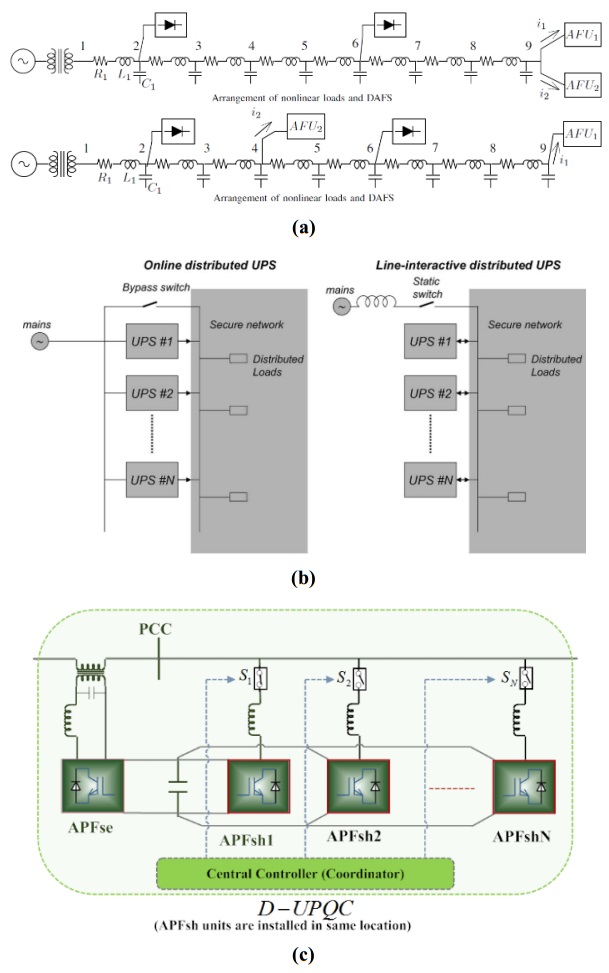
Cheng PT, Lee TL (2006) Distributed active filter systems (DAFSs): A new approach to power system harmonics. IEEE T Ind Appl 42: 1301–1309. doi: 10.1109/TIA.2006.880856
![]() |
[11] |
Guerrero JM, Hang L, Uceda J (2008) Control of distributed uninterruptible power supply systems. IEEE T Ind Electron 55: 2845–2859. doi: 10.1109/TIE.2008.924173
![]() |
[12] |
Lai J, Peng FZ (1996) Multilevel converters-a new breed of power converters. IEEE T Ind Appl 32: 509–517. doi: 10.1109/28.502161
![]() |
[13] |
Munoz JA, Espinoza JR, Moran LA, et al. (2009) Design of a modular UPQC configuration integrating a components economical analysis. IEEE T Power Deliver 24: 1763–1772. doi: 10.1109/TPWRD.2009.2028795
![]() |
[14] |
Peng FZ, Mckeever JW, Adams DJ (1998) A power line conditioner using cascade multilevel inverters for distribution systems. IEEE T Ind Appl 34: 1293–1298. doi: 10.1109/28.739012
![]() |
[15] |
Han B, Bae B, Baek S, et al. (2006) New configuration of UPQC for medium-voltage application. IEEE T Power Deliver 21: 1438–1444. doi: 10.1109/TPWRD.2005.860235
![]() |
[16] | Han B, Baek S, Kim H, et al. (2006) Dynamic characteristic analysis of SSSC based on multibridge inverter. IEEE Power Eng Rev 22: 62–63. |
[17] |
Han BM, Mattavelli P (2003) Operation analysis of novel UPFC based on 3-level half-bridge modules. IEEE Power Tech Conference Proceedings, Bologna. IEEE 4: 307–312. doi: 10.1109/PTC.2003.1304740
![]() |
[18] | Munoz JA, Espinoza JR, Baier CR, et al. (2011) Design of a discrete-time linear control strategy for a multi-cell UPQC. IEEE T Ind Electron 59: 3797–3807. |
[19] | Khadem MSK, Basu M, Conlon MF (2012) UPQC for power quality improvement in dg integrated smart grid network-a review. Int J Emerg Electr Power Syst 13: 3. |
[20] |
Basu M, Das SP, Dubey GK (2008) Investigation on the performance of UPQC-Q for voltage sag mitigation and power quality improvement at a critical load point. IET Gener Transm Dis 2: 414–423. doi: 10.1049/iet-gtd:20060317
![]() |
[21] |
Khadem S, Basu M, Conlon M (2014) Harmonic power compensation capacity of shunt apf and its relationship to design parameters. IET Power Electron 7: 418–430. doi: 10.1049/iet-pel.2013.0098
![]() |
[22] |
Corradini L, Mattavelli P, Corradin M, et al. (2010) Analysis of parallel operation of uninterruptible power supplies loaded through long wiring cables. IEEE T Power Electr 25: 1046–1054. doi: 10.1109/TPEL.2009.2031178
![]() |
[23] |
Guerrero JM, Matas J, Castilla M, et al. (2006) Wireless-control strategy for parallel operation of distributed-generation inverters. IEEE T Ind Electron 53: 1461–1470. doi: 10.1109/TIE.2006.882015
![]() |
[24] | Khadem SK, Basu M, Conlon MF (2011) A review of parallel operation of active power filters in the distributed generation system. European Conference on Power Electronics and Applications. IEEE, 1–10. |
[25] | Arrillaga J, Liu YH, Watson NR (2007) Self-commutating conversion, in flexible power transmission: The HVDC options. John Wiley & Sons, Ltd, Chichester, UK. |
[26] | Khadem SK, Basu M, Conlon MF (2013) Selection of design parameters to reduce the zero-sequence circulating current flow in parallel operation of DC linked multiple shunt APF units. Adv Power Electron 2013: 13. |
[27] |
Asiminoaei L, Aeloiza E, Enjeti PN, et al. (2008) Shunt active-power-filter topology based on parallel interleaved inverters. IEEE T Ind Electron 55: 1175–1189. doi: 10.1109/TIE.2007.907671
![]() |
[28] |
Chen TP (2012) Zero-sequence circulating current reduction method for parallel HEPWM inverters between AC bus and DC bus. IEEE T Ind Electron 59: 290–300. doi: 10.1109/TIE.2011.2106102
![]() |
[29] | Ye Z, Boroyevich D, Choi JY, et al. (2006) Control of circulating current in parallel three-phase boost rectifiers. Applied Power Electronics Conference and Exposition, 2000. IEEE 1: 506–512. |
[30] |
Chen TP (2006) Circulating zero-sequence current control of parallel three-phase inverters. IEE P-Elect Pow Appl 153: 282–288. doi: 10.1049/ip-epa:20050231
![]() |
[31] | Abdelli Y, Machmoum M, Khoor MS (2004) Control of a multi module parallel able three phase active power filters. International Conference on Harmonics and Quality of Power. IEEE, 543–548. |
[32] | Wei X, Dai K, Fang X, et al. (2006) Parallel control of three-phase three-wire shunt active power filters. Automat Electr Power Syst 31: 70–74. |
1. | Min Yang, Qiangyi Li, Information Security Risk Management Model for Big Data, 2022, 2022, 1687-5699, 1, 10.1155/2022/3383251 | |
2. | Shan Zhao, Kaibo Shi, Interpolation Functions Of General Type-2 Fuzzy Systems, 2024, 1562-2479, 10.1007/s40815-024-01872-3 | |
3. | Gerardo Maximiliano Méndez, Ismael López-Juárez, María Aracelia Alcorta García, Dulce Citlalli Martinez-Peon, Pascual Noradino Montes-Dorantes, The Enhanced Wagner–Hagras OLS–BP Hybrid Algorithm for Training IT3 NSFLS-1 for Temperature Prediction in HSM Processes, 2023, 11, 2227-7390, 4933, 10.3390/math11244933 | |
4. | Ritu Raj, One-dimensional input space modelling of a simplified general type-2 Mamdani and Takagi–Sugeno Fuzzy Proportional Integral Derivative controller, 2025, 147, 09521976, 110289, 10.1016/j.engappai.2025.110289 | |
5. | Mohamed Amine Hartani, Aissa Benhammou, Abdallah Laidi, 2025, 10.5772/intechopen.1006834 |
P1 | PID | T1F-PID | IT2F-PID | SGT2F-PID | ||
case 1 | ts(s) | 12.3 | 6.1 | 6.69 | 4.96 | |
tr(s) | 5.05 | 2.01 | 2.3 | 2.07 | ||
OS (%) | 5.1 | 22.2 | 19.1 | 14.9 | ||
ISE | 1.44 | 1.15 | 1.24 | 1.13 | ||
ITSE | 1.49 | 0.84 | 0.96 | 0.74 | ||
ITAE | 5.37 | 2.23 | 2.53 | 1.58 | ||
case 2 | ts(s) | 17.68 | 8.5 | 9.3 | 7.01 | |
tr(s) | 3.18 | 1.84 | 2.07 | 1.88 | ||
OS (%) | 29.8 | 39.2 | 35.1 | 28.0 | ||
ISE | 1.59 | 1.26 | 1.32 | 1.15 | ||
ITSE | 3.27 | 1.26 | 1.35 | 0.87 | ||
ITAE | 14.77 | 4.07 | 4.49 | 2.55 | ||
Case3 | ts(s) | > 20 | 9.18 | 9.72 | 7.95 | |
tr(s) | > 20 | 1.94 | 2.25 | 2.01 | ||
OS (%) | - | 17.8 | 11.7 | 11.0 | ||
ISE | 1.74 | 1.13 | 1.21 | 1.11 | ||
ITSE | 3.78 | 0.86 | 0.93 | 0.76 | ||
ITAE | 20.26 | 2.98 | 3.04 | 2.27 | ||
case 4 | ts(s) | > 20 | 8.85 | 9.61 | 8.0 | |
tr(s) | 12.06 | 3.05 | 3.59 | 3.06 | ||
OS (%) | 2.3 | 9.9 | 9.9 | 7.1 | ||
ISE | 2.67 | 1.47 | 1.61 | 1.46 | ||
ITSE | 5.73 | 1.30 | 1.60 | 1.23 | ||
ITAE | 17.08 | 3.87 | 4.77 | 3.10 |
P2 | PID | T1F-PID | IT2F-PID | SGT2F-PID | ||
case 1 | ts(s) | 22.9 | 9.36 | 10.49 | 3.94 | |
tr(s) | 1.78 | 2.0 | 2.31 | 2.49 | ||
OS (%) | 16.7 | 27.9 | 28.2 | 5.2 | ||
ISE | 0.71 | 1.09 | 1.23 | 1.09 | ||
ITSE | 1.53 | 0.96 | 1.23 | 0.72 | ||
ITAE | 16.02 | 3.62 | 4.70 | 1.37 | ||
case 2 | ts(s) | 22.71 | 13.44 | 14.91 | 9.72 | |
tr(s) | 1.56 | 1.95 | 2.2 | 2.14 | ||
OS (%) | 19.1 | 44.9 | 46.9 | 30.5 | ||
ISE | 0.90 | 1.44 | 1.60 | 1.26 | ||
ITSE | 1.64 | 1.92 | 2.51 | 1.10 | ||
ITAE | 15.86 | 7.56 | 10.00 | 3.77 | ||
case 3 | ts(s) | 26.3 | 18.33 | 19.76 | 8.14 | |
tr(s) | 3.37 | 2.62 | 3.01 | 2.96 | ||
OS (%) | 20.4 | 43.5 | 40.04 | 17.01 | ||
ISE | 1.27 | 1.78 | 1.91 | 1.44 | ||
ITSE | 4.13 | 3.63 | 4.02 | 1.36 | ||
ITAE | 29.76 | 15.44 | 17.88 | 3.69 | ||
case 4 | ts(s) | 20.94 | 9.25 | 12.28 | 5.68 | |
tr(s) | 1.71 | 1.98 | 2.27 | 2.25 | ||
OS (%) | 12.8 | 35.3 | 36.2 | 16.7 | ||
ISE | 0.75 | 1.27 | 1.41 | 1.17 | ||
ITSE | 0.96 | 1.30 | 1.65 | 0.82 | ||
ITAE | 11.26 | 4.60 | 6.28 | 1.84 |
P3 | PID | T1F-PID | IT2F-PID | SGT2F-PID | ||
case 1 | ts(s) | 6.32 | 2.69 | 2.91 | 0.52 | |
tr(s) | 1.41 | 0.62 | 0.69 | 0.6 | ||
OS (%) | 16.3 | 21.9 | 20.6 | 13.1 | ||
ISE | 0.52 | 0.28 | 0.31 | 0.25 | ||
ITSE | 0.26 | 0.07 | 0.08 | 0.04 | ||
ITAE | 1.34 | 0.33 | 0.38 | 0.15 | ||
case 2 | ts(s) | 6.65 | 4.08 | 4.34 | 2.84 | |
tr(s) | 1.42 | 0.61 | 0.69 | 0.58 | ||
OS (%) | 20.1 | 38.5 | 34.0 | 27.2 | ||
ISE | 0.62 | 0.41 | 0.43 | 0.34 | ||
ITSE | 0.36 | 0.16 | 0.16 | 0.08 | ||
ITAE | 1.73 | 0.64 | 0.7 | 0.30 | ||
case 3 | ts(s) | 7.52 | 3.15 | 3.44 | 2.07 | |
tr(s) | 1.3 | 0.6 | 0.67 | 0.58 | ||
OS (%) | 22.6 | 27.2 | 26.0 | 16.1 | ||
ISE | 0.54 | 0.29 | 0.33 | 0.25 | ||
ITSE | 0.33 | 0.09 | 0.11 | 0.04 | ||
ITAE | 1.93 | 0.43 | 0.51 | 0.18 | ||
case 4 | ts(s) | 2.73 | 2.19 | 2.37 | 1.56 | |
tr(s) | 1.27 | 0.53 | 0.6 | 0.55 | ||
OS (%) | 5.7 | 12.1 | 11.1 | 4.1 | ||
ISE | 0.36 | 0.21 | 0.23 | 0.20 | ||
ITSE | 0.10 | 0.03 | 0.04 | 0.02 | ||
ITAE | 0.33 | 0.15 | 0.17 | 0.07 |
P4 | IT2F-PID [80] | IT2F-PD+I [81] | PID | T1F-PID | IT2F-PID | SGT2F-PID | ||
case 1 | ISE | 0.036 | - | 2.78 × 10⁻⁴ | 3.32 × 10⁻⁴ | 2.53 × 10⁻⁴ | 1.9 × 10⁻⁴ | |
ITSE | - | - | 2.34 × 10⁻⁵ | 2.0 × 10⁻⁵ | 7.22 × 10⁻⁶ | 3.64 × 10⁻⁶ | ||
ITAE | - | - | 0.0036 | 9.35 × 10⁻⁴ | 4.52 × 10⁻⁴ | 1.62 × 10⁻⁴ | ||
RMSE | 0.0085 | - | 0.0118 | 0.0129 | 0.013 | 0.0097 | ||
IAE | 1.8001 | - | 0.0101 | 0.0076 | 0.0051 | 0.0033 | ||
case 2 | ISE | - | 1.5844 | 0.0045 | 0.0064 | 0.0069 | 0.005 | |
ITSE | - | - | 3.33 × 10⁻⁴ | 2.34 × 10⁻⁴ | 2.43 × 10⁻⁴ | 1.23 × 10⁻⁴ | ||
ITAE | - | - | 0.0119 | 0.003 | 0.0029 | 0.0014 | ||
RMSE | - | 0.0514 | 0.0472 | 0.0568 | 0.0586 | 0.0499 | ||
IAE | - | 7.4692 | 0.0379 | 0.029 | 0.0287 | 0.0191 |
P4 | IT2F-PD+I [81] | PID | T1F-PID | IT2F-PID | SGT2F-PID | ||
case 3 | ISE | 1.9203 | 0.0045 | 0.0064 | 0.0069 | 0.005 | |
ITSE | - | 3.56 × 10⁻⁴ | 2.34 × 10⁻⁴ | 2.43 × 10⁻⁴ | 1.25 × 10⁻⁴ | ||
ITAE | - | 0.0288 | 0.0035 | 0.0037 | 0.0019 | ||
RMSE | 0.04 | 0.0273 | 0.0328 | 0.0338 | 0.0288 | ||
IAE | 14.7056 | 0.0419 | 0.0292 | 0.0290 | 0.0192 | ||
case 4 | ISE | 2.527 | 0.0046 | 0.0066 | 0.007 | 0.0051 | |
ITSE | - | 6.47 × 10⁻⁴ | 5.9 × 10⁻⁴ | 5.5 × 10⁻⁴ | 4.0 × 10⁻⁴ | ||
ITAE | - | 0.0316 | 0.0172 | 0.0154 | 0.011 | ||
RMSE | 0.0649 | 0.0276 | 0.0331 | 0.0341 | 0.0291 | ||
IAE | 13.3876 | 0.044 | 0.033 | 0.032 | 0.022 | ||
case 5 | ISE | 0.094 | 2.78 × 10⁻⁴ | 3.32 × 10⁻⁴ | 2.53 × 10⁻⁴ | 1.90 × 10⁻⁴ | |
ITSE | - | 2.34 × 10⁻⁵ | 2.04 × 10⁻⁵ | 7.73 × 10⁻⁶ | 3.64 × 10⁻⁶ | ||
ITAE | - | 0.0036 | 0.0010 | 5.08 × 10⁻⁴ | 1.89 × 10⁻⁴ | ||
RMSE | 0.0125 | 0.0068 | 0.0074 | 0.0065 | 0.0056 | ||
IAE | 2.2475 | 0.0101 | 0.0077 | 0.0052 | 0.0033 | ||
case 6 | ISE | - | 0.0046 | 0.0065 | 0.0069 | 0.005 | |
ITSE | - | 7.53 × 10⁻⁴ | 3.67 × 10⁻⁴ | 3.79 × 10⁻⁴ | 1.75 × 10⁻⁴ | ||
ITAE | - | 0.0447 | 0.0169 | 0.0185 | 0.0091 | ||
RMSE | - | 0.0278 | 0.0329 | 0.0340 | 0.0289 | ||
IAE | - | 0.0508 | 0.0345 | 0.0347 | 0.022 |