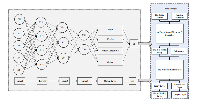
In recent years, automatic fault diagnosis for various machines has been a hot topic in the industry. This paper focuses on permanent magnet synchronous generators and combines fuzzy decision theory with deep learning for this purpose. Thus, a fuzzy neural network-based automatic fault diagnosis method for permanent magnet synchronous generators is proposed in this paper. The particle swarm algorithm optimizes the smoothing factor of the network for the effect of probabilistic neural network classification, as affected by the complexity of the structure and parameters. And on this basis, the fuzzy C means algorithm is used to obtain the clustering centers of the fault data, and the network model is reconstructed by selecting the samples closest to the clustering centers as the neurons in the probabilistic neural network. The mathematical analysis and derivation of the T-S (Tkagi-Sugneo) fuzzy neural network-based diagnosis strategy are carried out; the T-S fuzzy neural network-based generator fault diagnosis system is designed. The model is implemented on the MATLAB/Simulink platform for simulation and verification, the experiments show that the T-S fuzzy diagnosis strategy is significantly improved, and the design purpose is achieved. The fuzzy neural network has a parallel structure and can perform parallel data processing. This parallel mechanism can solve the problem of large-scale real-time computation in control systems, and the redundancy in parallel computation can make the control system highly fault-tolerant and robust. The fault diagnosis model based on an improved probabilistic neural network is applied to the fault data to verify the effectiveness and accuracy of the model.
Citation: Xueyan Wang. A fuzzy neural network-based automatic fault diagnosis method for permanent magnet synchronous generators[J]. Mathematical Biosciences and Engineering, 2023, 20(5): 8933-8953. doi: 10.3934/mbe.2023392
In recent years, automatic fault diagnosis for various machines has been a hot topic in the industry. This paper focuses on permanent magnet synchronous generators and combines fuzzy decision theory with deep learning for this purpose. Thus, a fuzzy neural network-based automatic fault diagnosis method for permanent magnet synchronous generators is proposed in this paper. The particle swarm algorithm optimizes the smoothing factor of the network for the effect of probabilistic neural network classification, as affected by the complexity of the structure and parameters. And on this basis, the fuzzy C means algorithm is used to obtain the clustering centers of the fault data, and the network model is reconstructed by selecting the samples closest to the clustering centers as the neurons in the probabilistic neural network. The mathematical analysis and derivation of the T-S (Tkagi-Sugneo) fuzzy neural network-based diagnosis strategy are carried out; the T-S fuzzy neural network-based generator fault diagnosis system is designed. The model is implemented on the MATLAB/Simulink platform for simulation and verification, the experiments show that the T-S fuzzy diagnosis strategy is significantly improved, and the design purpose is achieved. The fuzzy neural network has a parallel structure and can perform parallel data processing. This parallel mechanism can solve the problem of large-scale real-time computation in control systems, and the redundancy in parallel computation can make the control system highly fault-tolerant and robust. The fault diagnosis model based on an improved probabilistic neural network is applied to the fault data to verify the effectiveness and accuracy of the model.

| [1] |
K. Zhou, J. Tang, Harnessing fuzzy neural network for gear fault diagnosis with limited data labels, Int. J. Adv. Manuf. Technol., 115 (2021), 1005–1019. https://doi.org/10.1007/s00170-021-07253-6 doi: 10.1007/s00170-021-07253-6

|
| [2] |
R. Li, J. Chen, X. Wu, Fault diagnosis of rotating machinery using knowledge-based fuzzy neural network, Appl. Math. Mech., 27 (2006), 99–108. https://doi.org/10.1007/s10483-006-0113-1 doi: 10.1007/s10483-006-0113-1
|
| [3] |
M. Alexandru, Analysis of induction motor fault diagnosis with fuzzy neural network, Appl. Artif. Intell., 17 (2003), 105–133. https://doi.org/10.1080/713827102 doi: 10.1080/713827102
|
| [4] |
J. Luo, J. Huang, H. Li, A case study of conditional deep convolutional generative adversarial networks in machine fault diagnosis, J. Intell. Manuf., 32 (2021), 407–425. https://doi.org/10.1007/s10845-020-01579-w doi: 10.1007/s10845-020-01579-w
|
| [5] |
K. Zhou, E. Diehl, J. Tang, Deep convolutional generative adversarial network with semi-supervised learning enabled physics elucidation for extended gear fault diagnosis under data limitations, Mech. Syst. Signal Process., 185 (2023), 109772. https://doi.org/10.1016/j.ymssp.2022.109772 doi: 10.1016/j.ymssp.2022.109772
|
| [6] |
Y. He, H. Tang, Y. Ren, A. Kumar, A semi-supervised fault diagnosis method for axial piston pump bearings based on DCGAN, Meas. Sci. Technol., 32 (2021), 125104. https://doi.org/10.1088/1361-6501/ac1fbe doi: 10.1088/1361-6501/ac1fbe
|
| [7] |
Z. Guo, K. Yu, A. K. Bashir, D. Zhang, Y. D. Al-Otaibi, M. Guizani, Deep information fusion-driven POI scheduling for mobile social networks, IEEE Network, 36 (2022), 210–216. https://doi.org/10.1109/MNET.102.2100394 doi: 10.1109/MNET.102.2100394
|
| [8] |
L. Yang, Y. Li, S. X. Yang, Y. Lu, T. Guo, K. Yu, Generative adversarial learning for intelligent trust management in 6G wireless networks, IEEE Network, 36 (2022), 134–140. https://doi.org/10.1109/MNET.003.2100672 doi: 10.1109/MNET.003.2100672
|
| [9] |
Z. Guo, K. Yu, N. Kumar, W. Wei, S. Mumtaz, M. Guizani, Deep distributed learning-based POI recommendation under mobile edge networks, IEEE Internet Things J., 10 (2023), 303–317. https://doi.org/10.1109/JIOT.2022.3202628 doi: 10.1109/JIOT.2022.3202628
|
| [10] |
Z. Zhou, Y. Su, J. Li, K. Yu, Q. M. J. Wu, Z. Fu, et al., Secret-to-image reversible transformation for generative steganography, IEEE Trans. Dependable Secure Comput., 2022 (2022), 1–17. https://doi.org/10.1109/TDSC.2022.3217661 doi: 10.1109/TDSC.2022.3217661
|
| [11] | L. Zhao, Z. Bi, A. Hawbani, K. Yu, Y. Zhang, M. Guizani, ELITE: An intelligent digital twin-based hierarchical routing scheme for softwarized vehicular networks, IEEE Trans. Mobile Comput., 2022 (2022). https://doi.org/10.1109/TMC.2022.3179254 |
| [12] |
A. Rohan, S. H. Kim, RLC fault detection based on image processing and artificial neural network, Int. J. Fuzzy Logic Intell. Syst., 19 (2019), 78–87. https://doi.org/10.5391/IJFIS.2019.19.2.78 doi: 10.5391/IJFIS.2019.19.2.78
|
| [13] |
I. Jlassi, A. J. M. Cardoso, A single method for multiple IGBT, current, and speed sensor faults diagnosis in regenerative PMSM drives, IEEE J. Emerging Sel. Top. Power Electron., 8 (2019), 2583–2599. https://doi.org/10.1109/JESTPE.2019.2918062 doi: 10.1109/JESTPE.2019.2918062
|
| [14] |
D. T. Hoang, H. J. Kang, A motor current signal-based bearing fault diagnosis using deep learning and information fusion, IEEE Trans. Instrum. Meas., 69 (2019), 3325–3333. https://doi.org/10.1109/TIM.2019.2933119 doi: 10.1109/TIM.2019.2933119
|
| [15] |
E. A. Bhuiyan, M. M. A. Akhand, S. K. Das, M. F. Ali, Z. Tasneem, Md. R. Islam, et al., A survey on fault diagnosis and fault tolerant methodologies for permanent magnet synchronous machines, Int. J. Autom. Comput., 17 (2020), 763–787. https://doi.org/10.1007/s11633-020-1250-3 doi: 10.1007/s11633-020-1250-3
|
| [16] |
Z. Ullah, S. T. Lee, J. Hur, A torque angle-based fault detection and identification technique for IPMSM, IEEE Trans. Ind. Appl., 56 (2019), 170–182. https://doi.org/10.1109/TIA.2019.2947401 doi: 10.1109/TIA.2019.2947401
|
| [17] |
Y. Zou, Y. Zhang, H. Mao, Fault diagnosis on the bearing of traction motor in high-speed trains based on deep learning, Alexandria Eng. J., 60 (2021), 1209–1219. https://doi.org/10.1016/j.aej.2020.10.044 doi: 10.1016/j.aej.2020.10.044
|
| [18] |
G. Rigatos, N. Zervos, M. Abbaszadeh, P. Siano, D. Serpanose, V. Siadimas, Neural networks and statistical decision making for fault diagnosis of PM linear synchronous machines, Int. J. Syst. Sci., 51 (2020), 2150–2166. https://doi.org/10.1080/00207721.2020.1792579 doi: 10.1080/00207721.2020.1792579
|
| [19] |
S. Zhang, H. Zhao, J. Xu, W. Deng, A novel fault diagnosis method based on improved adaptive variational mode decomposition, energy entropy, and probabilistic neural network, Trans. Can. Soc. Mech. Eng., 44 (2019), 121–132. https://doi.org/10.1139/tcsme-2018-0195 doi: 10.1139/tcsme-2018-0195
|
| [20] |
P. Zhang, Z. Cui, Y. Wang, S. Ding, Application of BPNN optimized by chaotic adaptive gravity search and particle swarm optimization algorithms for fault diagnosis of electrical machine drive system, Electr. Eng., 104 (2022), 819–831. https://doi.org/10.1007/s00202-021-01335-0 doi: 10.1007/s00202-021-01335-0
|
| [21] |
F. Raj, V. K. Kannan, Particle swarm optimized deep convolutional neural sugeno-takagi fuzzy PID controller in permanent magnet synchronous motor, Int. J. Fuzzy Syst., 24 (2022), 180–201. https://doi.org/10.1007/s40815-021-01126-6 doi: 10.1007/s40815-021-01126-6
|
| [22] |
M. A. Saeed, M. El-Saadawi, Practical implementation and testing of RNN based synchronous generator internal-fault protection, Recent Pat. Electr. Electron. Eng., 12 (2019), 181–189. https://doi.org/10.2174/2352096511666180605095153 doi: 10.2174/2352096511666180605095153
|
| [23] |
S. Lu, R. Yan, Y. Liu, Q. Wang, Tacholess speed estimation in order tracking: A review with application to rotating machine fault diagnosis, IEEE Trans. Instrum. Meas., 68 (2019), 2315–2332. https://doi.org/10.1109/TIM.2019.2902806 doi: 10.1109/TIM.2019.2902806
|
| [24] |
M. Xue, H. Yan, M. Wang, H. Shen, K. Shi, LSTM-based intelligent fault detection for fuzzy Markov jump systems and its application to tunnel diode circuits, IEEE Trans. Circuits Syst. II Express Briefs, 69 (2021), 1099–1103. https://doi.org/10.1109/TCSII.2021.3092627 doi: 10.1109/TCSII.2021.3092627
|
| [25] |
F. F. M. El-Sousy, M. M. Amin, O. A. Mohammed, Robust optimal control of high–speed permanent–magnet synchronous motor drives via self-constructing fuzzy wavelet neural network, IEEE Trans. Ind. Appl., 57 (2020), 999–1013. https://doi.org/10.1109/TIA.2020.3035131 doi: 10.1109/TIA.2020.3035131
|
| [26] |
S. Lu, G. Qian, Q. He, F. Liu, Y. Liu, Q. Wang, In situ motor fault diagnosis using enhanced convolutional neural network in an embedded system, IEEE Sensors J., 20 (2019), 8287–8296. https://doi.org/10.1109/JSEN.2019.2911299 doi: 10.1109/JSEN.2019.2911299
|
| [27] |
A. Abid, M. T. Khan, J. Iqbal, A review on fault detection and diagnosis techniques: basics and beyond, Artif. Intell. Rev., 54 (2021), 3639–3664. https://doi.org/10.1007/s10462-020-09934-2 doi: 10.1007/s10462-020-09934-2
|
| [28] |
S. Li, H. Won, X. Fu, M. Fairbank, D. C. Wunsch, E. Alonso, Neural-network vector controller for permanent–magnet synchronous motor drives: Simulated and hardware-validated results, IEEE Trans. Cybern., 50 (2019), 3218–3230. https://doi.org/10.1109/TCYB.2019.2897653 doi: 10.1109/TCYB.2019.2897653
|
| [29] |
F. Wan, X. Miao, B. Ravelo, Q. Yuan, J. Cheng, Q. Ji, et al., Design of multi–scale negative group delay circuit for sensors signal time–delay cancellation, IEEE Sensors J., 19 (2019), 8951–8962. https://doi.org/10.1109/JSEN.2019.2921834 doi: 10.1109/JSEN.2019.2921834
|
| [30] |
X. Shen, G. Shi, H. Ren, W. Zhang, Biomimetic vision for zoom object detection based on improved vertical grid number YOLO algorithm, Front. Bioeng. Biotechnol., 10 (2022), 905583. https://doi.org/10.3389/fbioe.2022.905583 doi: 10.3389/fbioe.2022.905583
|
| [31] |
L. Chen, W. Li, Y. Yang, W. Miao, Evaluation and optimization of vehicle pedal comfort based on biomechanics, Proc. Inst. Mech. Eng. Part D, 234 (2020), 1402–1412. https://doi.org/10.1177/0954407019878355 doi: 10.1177/0954407019878355
|
| [32] |
Z. Guo, K. Yu, A. Jolfaei, F. Ding, N. Zhang, Fuz-Spam: Label smoothing-based fuzzy detection of spammers in internet of things, IEEE Trans. Fuzzy Syst., 30 (2022), 4543–4554. https://doi.org/10.1109/TFUZZ.2021.3130311 doi: 10.1109/TFUZZ.2021.3130311
|
| [33] | L. Zhao, Z. Yin, K. Yu, X. Tang, L. Xu, Z. Guo, et al., A fuzzy logic based intelligent multi-attribute routing scheme for two-layered SDVNs, IEEE Trans. Network Serv. Manage., 2022 (2022). https://doi.org/10.1109/TNSM.2022.3202741 |
| [34] |
Z. Guo, Y. Shen, S. Wan, W. Shang, K. Yu, Hybrid intelligence-driven medical image recognition for remote patient diagnosis in internet of medical things, IEEE J. Biomed. Health Inf., 26 (2022), 5817–5828. https://doi.org/10.1109/JBHI.2021.3139541 doi: 10.1109/JBHI.2021.3139541
|
| [35] |
C. Chen, Z. Liao, Y. Ju, C. He, K. Yu, S. Wan, Hierarchical domain-based multi-controller deployment strategy in SDN-enabled space-air-ground integrated network, IEEE Trans. Aerospace Electron. Syst., 58 (2022), 4864–4879. https://doi.org/10.1109/TAES.2022.3199191 doi: 10.1109/TAES.2022.3199191
|
| [36] | Z. Zhou, Y. Li, J. Li, K. Yu, G. Kou, M. Wang, et al., Gan-siamese network for cross-domain vehicle re-identification in intelligent transport systems, IEEE Trans. Network Sci. Eng., 2022 (2022). https://doi.org/10.1109/TNSE.2022.3199919 |
Figures(8) / Tables(2)

Xueyan Wang. A fuzzy neural network-based automatic fault diagnosis method for permanent magnet synchronous generators[J]. Mathematical Biosciences and Engineering, 2023, 20(5): 8933-8953. doi: 10.3934/mbe.2023392


 DownLoad: