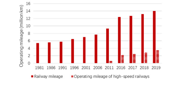
After decades of rapid development, economic level has undergone qualitative changes in both aggregate and structural terms in China. This paper introduces the concept of market access, which argues that there are externalities to the opening of high-speed railways (HSRs) and that the accessibility of cities without high-speed railways is similarly affected by the opening of high-speed railways in other cities and investigates the impact of the opening of high-speed railways on the market access of cities. By drawing on Herzog's estimation framework, general equilibrium conditions for trade are estimated and a derived simplified model is used to determine a method for measuring cities' ability to enter the market. A systematic study of the market access indicator methodology for assessing transport infrastructure improvements is conducted to examine the spatial and temporal evolution of high-speed rail construction in China, measure the changes in market access due to high-speed rail and conduct a characteristic factual analysis based on the results obtained. The paper finds that the average inter-city travel time in China fell by 2.27 hours, i.e., 15.67%, from 2015 to 2019, with the marginal contribution to the decline in travel time coming mainly from the opening of HSRs. Over the 10 years from 2010 to 2019, the logarithm of access to market capacity for Chinese cities increased by around 50%, with the construction of high-speed railways leading to a substantial increase in access to market capacity. Overall, this paper focuses on the scientific method of measurement to provide a better objective understanding of the impact and evolution of high-speed rail construction on the market access of cities in China.
Citation: Shuchang Yi, Qing Liu, Yanze Zhang. High-speed rail construction and market access of cities: Empirical evidence from China[J]. Urban Resilience and Sustainability, 2023, 1(3): 146-162. doi: 10.3934/urs.2023011
After decades of rapid development, economic level has undergone qualitative changes in both aggregate and structural terms in China. This paper introduces the concept of market access, which argues that there are externalities to the opening of high-speed railways (HSRs) and that the accessibility of cities without high-speed railways is similarly affected by the opening of high-speed railways in other cities and investigates the impact of the opening of high-speed railways on the market access of cities. By drawing on Herzog's estimation framework, general equilibrium conditions for trade are estimated and a derived simplified model is used to determine a method for measuring cities' ability to enter the market. A systematic study of the market access indicator methodology for assessing transport infrastructure improvements is conducted to examine the spatial and temporal evolution of high-speed rail construction in China, measure the changes in market access due to high-speed rail and conduct a characteristic factual analysis based on the results obtained. The paper finds that the average inter-city travel time in China fell by 2.27 hours, i.e., 15.67%, from 2015 to 2019, with the marginal contribution to the decline in travel time coming mainly from the opening of HSRs. Over the 10 years from 2010 to 2019, the logarithm of access to market capacity for Chinese cities increased by around 50%, with the construction of high-speed railways leading to a substantial increase in access to market capacity. Overall, this paper focuses on the scientific method of measurement to provide a better objective understanding of the impact and evolution of high-speed rail construction on the market access of cities in China.

| [1] |
Baum-Snow N (2007) Did highways cause suburbanization? Q J Econ 122: 775–805. https://doi.org/10.1162/qjec.122.2.775 doi: 10.1162/qjec.122.2.775

|
| [2] | Yuan J (2015) Responses of China's urban master planning under HSR effects. City Plan Rev 39: 19–24. |
| [3] | Zhang Y, Hua C (2011) HSR promote urban spatial restructuring as a structural element: A case study of Lyon. Urban Plan Int 26: 102–109. |
| [4] | Li W, Zhai G, He Z, et al. (2016) The enlightenment of the Japanese station-city development to the construction of high speed railway new town in China: A case study of the New Yokohama station. Urban Plan Int 31: 111–118. |
| [5] | Sands BD (1993). The development effect of high-speed rail stations and implications for California. Build Environ 19: 257–284. |
| [6] |
Vickerman R (1997) High-speed rail in Europe: Experience and issues for future development. Ann Reg Sci 31: 21–38. https://doi.org/10.1007/s001680050037 doi: 10.1007/s001680050037
|
| [7] | Jiang B, Chu N, Wang Y, et al. (2016) The research review and prospect of the impact on urban and regional space of high-speed rail. Hum Geogr 31: 16–25. |
| [8] | Yi S, Liu Q, Zhang Y (2023) High-speed railway operation and wage inequality of manufacturing enterprises within cities: Facts, mechanisms, and policy implications. J Lanzhou Univ Soc Sci 51: 13–25. Available from: https://10.13885/j.issn.1000-2804.2023.04.002. |
| [9] | Cao Y, Yu L, Li S (2020) Spatial evolution of high-speed railway station areas and planning response. City Plan Rev 44: 88–96. |
| [10] | Donaldson D, Hornbeck R (2016) Railroads and American economic growth: A "market access" approach. Q J Econ 131: 799–858. https://doi.org/10.1093/qje/qjw002 |
| [11] |
Lin Y (2017) Travel costs and urban specialization patterns: Evidence from China's high speed railway system. J Urban Econ 98: 98–123. https://doi.org/10.1016/j.jue.2016.11.002 doi: 10.1016/j.jue.2016.11.002
|
| [12] | Tang Y, Yu F, Lin F, et al. (2019) China's high-speed railway, trade cost and firm export. Econ Res 54: 158–173. |
| [13] |
Herzog I (2021) National transportation networks, market access, and regional economic growth. J Urban Econ 122: 103316. https://doi.org/10.1016/j.jue.2020.103316 doi: 10.1016/j.jue.2020.103316
|
| [14] |
Eaton J, Kortum S (2002) Technology, geography, and trade. Econometrica 70: 1741–1779. https://doi.org/10.1111/1468-0262.00352 doi: 10.1111/1468-0262.00352
|
| [15] | Duranton G, Turner MA (2012) Urban growth and transportation. Rev Econ Stud 79(4): 1407–1440. https://doi.org/10.1093/restud/rds010 |
| [16] |
Allen T, Arkolakis C (2014) Trade and the topography of the spatial economy. Q J Econ 129: 1085–1140. https://doi.org/10.1093/qje/qju016 doi: 10.1093/qje/qju016
|
| [17] | Bartelme D (2015) Trade costs and economic geography: evidence from the us. Working Paper of University of California. |
| [18] |
Costinot A, Donaldson D, Komunjer I (2012) What goods do countries trade? A quantitative exploration of Ricardo's ideas. Rev Econ Stud 79: 581–608. https://doi.org/10.1093/restud/rdr033 doi: 10.1093/restud/rdr033
|
| [19] |
Simonovska I, Waugh ME (2014) The elasticity of trade: Estimates and evidence. J Int Econ 92: 34–50. https://doi.org/10.1016/j.jinteco.2013.10.001 doi: 10.1016/j.jinteco.2013.10.001
|
| [20] |
Bernard AB, Eaton J, Jensen JB, et al. (2003) Plants and productivity in international trade. Am Econ Rev 93: 1268–1290. https://doi.org/10.1257/000282803769206296 doi: 10.1257/000282803769206296
|
| [21] |
Tombe T, Zhu X (2019) Trade, migration, and productivity: a quantitative analysis of China. Am Econ Rev 109: 1843–1872. https://doi.org/10.1257/aer.20150811 doi: 10.1257/aer.20150811
|
| [22] | Xu M (2017) Riding on the new silk road: Quantifying the welfare gains from high-speed railways. Job Mark Pap 25: 32–40. |
| [23] | Zhang M, Yu F, Zhong CB, et al. (2018) High-speed railways, market access and enterprises' productivity. China Ind Econ 362: 137–156. Available from: https://10.19581/j.cnki.ciejournal.2018.05.008. |


Figures(6) / Tables(2)
Shuchang Yi, Qing Liu, Yanze Zhang. High-speed rail construction and market access of cities: Empirical evidence from China[J]. Urban Resilience and Sustainability, 2023, 1(3): 146-162. doi: 10.3934/urs.2023011


 DownLoad: