The Laplace transform is a popular approach in solving ordinary differential equations (ODEs), particularly solving initial value problems (IVPs) of ODEs. Such stereotype may confuse students when they face a task of solving ODEs without explicit initial condition(s). In this paper, four case studies of solving ODEs by the Laplace transform are used to demonstrate that, firstly, how much influence of the stereotype of the Laplace transform was on student's perception of utilizing this method to solve ODEs under different initial conditions; secondly, how the generalization of the Laplace transform for solving linear ODEs with generic initial conditions can not only break down the stereotype but also broaden the applicability of the Laplace transform for solving constant-coefficient linear ODEs. These case studies also show that the Laplace transform is even more robust for obtaining the specific solutions directly from the general solution once the initial values are assigned later. This implies that the generic initial conditions in the general solution obtained by the Laplace transform could be used as a point of control for some dynamic systems.
Citation: William Guo. The Laplace transform as an alternative general method for solving linear ordinary differential equations[J]. STEM Education, 2021, 1(4): 309-329. doi: 10.3934/steme.2021020
The Laplace transform is a popular approach in solving ordinary differential equations (ODEs), particularly solving initial value problems (IVPs) of ODEs. Such stereotype may confuse students when they face a task of solving ODEs without explicit initial condition(s). In this paper, four case studies of solving ODEs by the Laplace transform are used to demonstrate that, firstly, how much influence of the stereotype of the Laplace transform was on student's perception of utilizing this method to solve ODEs under different initial conditions; secondly, how the generalization of the Laplace transform for solving linear ODEs with generic initial conditions can not only break down the stereotype but also broaden the applicability of the Laplace transform for solving constant-coefficient linear ODEs. These case studies also show that the Laplace transform is even more robust for obtaining the specific solutions directly from the general solution once the initial values are assigned later. This implies that the generic initial conditions in the general solution obtained by the Laplace transform could be used as a point of control for some dynamic systems.

| [1] |
Kreyszig, E., Advanced Engineering Mathematics, 10th ed. 2011, USA: Wiley. |
| [2] |
Fatoorehchi, H. and Rach, R., A method for inverting the Laplace transform of two classes of rational transfer functions in control engineering. Alexandria Engineering Journal, 2020, 59: 4879-4887. |
| [3] |
Ha, W. and Shin C., Seismic random noise attenuation in the Laplace domain using SVD. IEEE Access, 2021, 9: 62037. |
| [4] |
Grasso, F., Manetti, S., Piccirilli, M.C. and Reatti, A., A Laplace transform approach to the simulation of DC-DC converters. International Journal of Numerical Modelling: Electronic Networks, Devices and Fields, 2019, 32(5): e2618. |
| [5] |
Han, H. and Kim, H., The solution of exponential growth and exponential decay by using Laplace transform. International Journal of Difference Equations, 2020, 15(2):191-195. |
| [6] |
Huang, L., Deng, L., Li, A., Gao, R., Zhang, L. and Lei, W., A novel approach for solar greenhouse air temperature and heating load prediction based on Laplace transform. Journal of Building Engineering, 2021, 44: 102682. |
| [7] |
Daci, A. and Tola, S., Laplace transform, application in population growth. International Journal of Recent Technology and Engineering, 2019, 8(2): 954-957. |
| [8] |
Etzweiler, G. and S. Steele., The Laplace transformation of the impulse function for engineering problems. IEEE Transactions on Education, 1967, 10: 171-173. |
| [9] |
Zill, D.G., A First Course in Differential Equations with Modeling Applications, 10th ed. 2013, Boston, USA: Cengage Learning. |
| [10] |
Nise, N.S. Control Systems Engineering, 8th ed. 2019, USA: John Wiley & Sons. |
| [11] |
AL-Khazraji, H., Cole, C. and Guo, W., Analysing the impact of different classical controller strategies on the dynamics performance of production-inventory systems using state space approach. Journal of Modelling in Management, 2018, 13(1): 211-235. https://doi.org/10.1108/JM2-08-2016-0071 doi: 10.1108/JM2-08-2016-0071
|
| [12] |
AL-Khazraji, H., Cole, C. and Guo, W., Optimization and simulation of dynamic performance of production–inventory systems with multivariable controls. Mathematics, 2021, 9(5): 568. https://doi.org/10.3390/math9050568 doi: 10.3390/math9050568
|
| [13] |
Guo, W.W., Advanced Mathematics for Engineering and Applied Sciences, 3rd ed. 2016, Sydney, Australia: Pearson. |
| [14] |
Ngo, V. and Ouzomgi, S., Teaching the Laplace transform using diagrams. The College Mathematics Journal, 1992, 23(4): 309-312. |
| [15] |
Holmberg, M. and Bernhard. J., University teachers' perspectives on the role of the Laplace transform in engineering education. European Journal of Engineering Education, 2017, 42(4): 413-428. https://doi.org/10.1080/03043797.2016.1190957 doi: 10.1080/03043797.2016.1190957
|
| [16] |
Croft, A. and Davison, R., Engineering Mathematics, 5th ed. 2019, Harlow, UK: Pearson. |
| [17] |
Greenberg, M.D., Advanced Engineering Mathematics. 2nd ed. 1998, Upper Saddle River, USA: Prentice Hall. |
| [18] |
James, G., Modern Engineering Mathematics, 2nd ed. 1996, Harlow, UK: Addison-Wesley Longman. |
| [19] |
Yeung, K.S. and Chung, W.D., On solving differential equations using the Laplace transform. International Journal of Electrical Engineering and Education. 2007, 44(4): 373-376. |
| [20] |
Robertson, R.L., Laplace transform without integration. PRIMUS, 2017, 27(6): 606–617. https://doi.org/10.1080/10511970.2016.1235643 doi: 10.1080/10511970.2016.1235643
|
| [21] |
Srivastava, H.M., Masjed-Jamei, M. and Aktas, R., Analytical solutions of some general classes of differential and integral equations by using the Laplace and Fourier transforms. Filomat, 2020, 34(9): 2869-2876. https://doi.org/10.2298/FIL2009869S doi: 10.2298/FIL2009869S
|
| [22] |
Guo, W., Unification of the common methods for solving the first-order linear ordinary differential equations. STEM Education, 2021, 1(2): 127-140. https://doi.org/10.3934/steme.2021010 doi: 10.3934/steme.2021010
|
| [23] |
Guo, W., Li, W. and Tisdell, C.C., Effective pedagogy of guiding undergraduate engineering students solving first-order ordinary differential equations. Mathematics, 2021, 9(14):1623. https://doi.org/10.3390/math9141623 doi: 10.3390/math9141623
|
| [24] |
Garner, B. and Garner, L., Retention of concepts and skills in traditional and reformed applied calculus. Mathematics Education Research Journal, 2001, 13: 165-184. |
| [25] |
Kwon, O.N., Rasmussen, C. and Allen, K., Students' retention of mathematical knowledge and skills in differential equations. School Science and Mathematics, 2005,105: 227-239. |


Figures(11) / Tables(2)
William Guo. The Laplace transform as an alternative general method for solving linear ordinary differential equations[J]. STEM Education, 2021, 1(4): 309-329. doi: 10.3934/steme.2021020

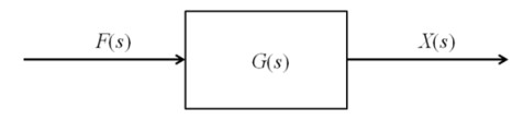
A system represented by a single block diagram in the state space
The series RL circuit with input
Electric currents in the RL circuit with R = 10 Ω, L = 5 H, ω = 2, and E0 = 10 V
Plot of the output for Case 2 with y(0) = 0 and y′(0) = 0
An example of student's work on solving the ODE in Case 2 by the Laplace transform
Plots of the solution to Case 3 with fixed y(0) = 1 and different values for
Electric currents of the RL circuit in Case 1 with R = 10 Ω, L = 5 H, ω = 2, and E0 = 10 V [v0 = i(0) for –10, 0, and 10 amperes, respectively]
Plots of the output of the ODE in Case 2 by Laplace transform with different initial values [Black: v0 = –3, v1 = –3; Red: v0 = 0, v1 = 0; Blue: v0 = 5, v1 = 5]
The mixing problem for Case 4
Plots of the mixing processes in the solutions (34) and (35) V = 4000 liters, x0 = 600 kg, y0 = 0 kg; blue curves: q1 = 40 l/m; red curves: q2 = 100 l/m
Plots of the mixing processes in the solutions (36) and (37) V = 4000 liters, x0 = 500 kg, y0 = 100 kg; blue curves: q1 = 40 l/m; red curves: q2 = 100 l/m


 DownLoad: