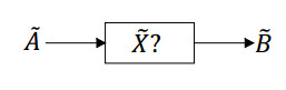
This paper mainly studied the problem of solving interval type-2 fuzzy relation equations $ \widetilde A \circ \widetilde X = \widetilde B $. First, to solve the interval type-2 fuzzy relation equations, we extend the semi-tensor product of matrices to interval matrices and give its specific definition. Second, the interval type-2 fuzzy relation equation was divided into two parts: primary fuzzy matrix equation $ {\widetilde A_\mu } \circ {\widetilde X_\mu }{\rm{ = }}{\widetilde B_\mu} $ and secondary fuzzy matrix equation $ {\widetilde A_f} \circ {\widetilde X_f} = {\widetilde B_f} $. Since all elements of $ {\widetilde X_f} $ equal to one, only the principal fuzzy matrix equation needs to be considered. Furthermore, it was proved that all solutions can be obtained from the parameter set solutions if the primary fuzzy matrix equation is solvable. Finally, with semi-tensor product of interval matrices, the primary fuzzy matrix equation was transformed into an algebraic equation and the specific algorithm for solving an interval type-2 fuzzy relation equation was proposed.
Citation: Aidong Ge, Zhen Chang, Jun-e Feng. Solving interval type-2 fuzzy relation equations via semi-tensor product of interval matrices[J]. Mathematical Modelling and Control, 2023, 3(4): 331-344. doi: 10.3934/mmc.2023027
This paper mainly studied the problem of solving interval type-2 fuzzy relation equations $ \widetilde A \circ \widetilde X = \widetilde B $. First, to solve the interval type-2 fuzzy relation equations, we extend the semi-tensor product of matrices to interval matrices and give its specific definition. Second, the interval type-2 fuzzy relation equation was divided into two parts: primary fuzzy matrix equation $ {\widetilde A_\mu } \circ {\widetilde X_\mu }{\rm{ = }}{\widetilde B_\mu} $ and secondary fuzzy matrix equation $ {\widetilde A_f} \circ {\widetilde X_f} = {\widetilde B_f} $. Since all elements of $ {\widetilde X_f} $ equal to one, only the principal fuzzy matrix equation needs to be considered. Furthermore, it was proved that all solutions can be obtained from the parameter set solutions if the primary fuzzy matrix equation is solvable. Finally, with semi-tensor product of interval matrices, the primary fuzzy matrix equation was transformed into an algebraic equation and the specific algorithm for solving an interval type-2 fuzzy relation equation was proposed.

| [1] |
L. A. Zadeh, Quantitative fuzzy semantics, Inf. Sci., 3 (1971), 159–176. https://doi.org/10.1016/S0020-0255(71)80004-X doi: 10.1016/S0020-0255(71)80004-X

|
| [2] |
L. A. Zadeh, The concept of a linguistic variable and its application to approximate reasoning-Ⅰ, Inf. Sci., 8 (1975), 199–249. https://doi.org/10.1016/0020-0255(75)90036-5 doi: 10.1016/0020-0255(75)90036-5
|
| [3] |
M. Mizumoto, K. Tanaka, Some properties of fuzzy sets of type 2, Inf. Control, 31 (1976), 312–340. https://doi.org/10.1016/S0019-9958(76)80011-3 doi: 10.1016/S0019-9958(76)80011-3
|
| [4] |
M. Mizumoto, K. Tanaka, Fuzzy sets and type 2 under algebraic product and algebraic sum, Fuzzy Set Syst., 5 (1981), 277–290. https://doi.org/10.1016/0165-0114(81)90056-7 doi: 10.1016/0165-0114(81)90056-7
|
| [5] |
N. N. Karnik, J. M. Mendel, Centroid of a type-2 fuzzy set, Inf. Sci., 132 (2001), 195–220. https://doi.org/10.1016/S0020-0255(01)00069-X doi: 10.1016/S0020-0255(01)00069-X
|
| [6] |
N. N. Karnik, J. M. Mendel, Introduction to type-2 fuzzy logic systems, 1998 IEEE International Conference on Fuzzy Systems Proceedings. IEEE World Congress on Computational Intelligence, 1998,915–920. https://doi.org/10.1109/FUZZY.1998.686240 doi: 10.1109/FUZZY.1998.686240
|
| [7] |
A. K. Das, S. Sundaram, Introduction to type-2 fuzzy logic systems, IEEE Trans. Fuzzy Syst., 24 (2016), 1565–1577. https://doi.org/10.1109/TFUZZ.2016.2540072 doi: 10.1109/TFUZZ.2016.2540072
|
| [8] |
V. Singh, R. Dev, N. K. Dhar, P. Agrawal, N. K. Verma, Adaptive type-2 fuzzy approach for filtering salt and pepper noise in grayscale images, IEEE Trans. Fuzzy Syst., 26 (2018), 3170–3176. https://doi.org/10.1109/TFUZZ.2018.2805289 doi: 10.1109/TFUZZ.2018.2805289
|
| [9] |
A. A. Molai, E. Khorram, An algorithm for solving fuzzy relation equations with max-$T$ composition operator, Inf. Sci., 178 (2008), 1293–1308. https://doi.org/10.1016/j.ins.2007.10.010 doi: 10.1016/j.ins.2007.10.010
|
| [10] | D. Dubois, H. Prade, Fundamentals of fuzzy sets, New York: Springer Science & Business Media, 2012. https://doi.org/10.1007/978-1-4615-4429-6 |
| [11] |
H. Lyu, W. Wang, X. Liu, Universal approximation of fuzzy relation models by semitensor product, IEEE Trans. Fuzzy Syst., 28 (2019), 2972–2981. https://doi.org/10.1109/TFUZZ.2019.2946512 doi: 10.1109/TFUZZ.2019.2946512
|
| [12] |
C. Sun, H. Li, Parallel fuzzy relation matrix factorization towards algebraic formulation, universal approximation and interpretability of MIMO hierarchical fuzzy systems, Fuzzy Set Syst., 450 (2022), 68–86. https://doi.org/10.1016/j.fss.2022.07.008 doi: 10.1016/j.fss.2022.07.008
|
| [13] |
C. Sun, H. Li, Algebraic formulation and application of multi-input single-output hierarchical fuzzy systems with correction factors, IEEE Trans. Fuzzy Syst., 31 (2023), 2076–2085. https://doi.org/10.1109/TFUZZ.2022.3220942 doi: 10.1109/TFUZZ.2022.3220942
|
| [14] |
Y. Yan, D. Cheng, J. E. Feng, H. Li, J. Yue, Survey on applications of algebraic state space theory of logical systems to finite state machines, Sci. China Inf. Sci., 66 (2023), 11201. https://doi.org/10.1007/s11432-022-3538-4 doi: 10.1007/s11432-022-3538-4
|
| [15] |
D. Cheng, J. E. Feng, H. Lv, Solving fuzzy relational equations via semi-tensor product, IEEE Trans. Fuzzy Syst., 20 (2012), 390–396. https://doi.org/10.1109/TFUZZ.2011.2174243 doi: 10.1109/TFUZZ.2011.2174243
|
| [16] |
J. F. Li, T. Li, W. Li, Y. M. Chen, R. Huang, Solvability of matrix equations $AX = B$, $XC = D$ under semi-tensor product, Linear Multilinear Algebra, 65 (2017), 1705–1733. https://doi.org/10.1080/03081087.2016.1253664 doi: 10.1080/03081087.2016.1253664
|
| [17] |
H. Fan, J. Feng, L. Zhang, Solving fuzzy relational equations via semi-tensor product, Proceedings of the 10th World Congress on Intelligent Control and Automation, 2012, 1465–1470. https://doi.org/10.1109/WCICA.2012.6358110 doi: 10.1109/WCICA.2012.6358110
|
| [18] |
S. Wang, H. Li, Resolution of fuzzy relational inequalities with Boolean semi-tensor product composition, Mathematics, 9 (2021), 937. https://doi.org/10.3390/math9090937 doi: 10.3390/math9090937
|
| [19] | Y. Yan, Z. Chen, Solving singleton type-2 fuzzy relation equations based on semi-tensor product of matrices, Proceedings of the 32nd Chinese Control Conference, 2013, 3434–3439. https://ieeexplore.ieee.org/abstract/document/6640015 |
| [20] |
Y. Yan, Z. Chen, Z. Liu, Solving type-2 fuzzy relation equations via semi-tensor product of matrices, Control Theory Technol., 12 (2014), 173–186. https://doi.org/10.1007/s11768-014-0137-7 doi: 10.1007/s11768-014-0137-7
|
| [21] | S. Z. Bo, Interval-valued fuzzy relation equations, Fuzzy Syst. Math., 1995. |
| [22] | L. Jaulin, M. Kieffer, O. Didrit, É. Walter, Interval analysis, London: Springer, 2001. https://doi.org/10.1007/978-1-4471-0249-6_2 |
| [23] |
A. Ge, Y. Wang, A. Wei, H. Liu, Control design for multi-variable fuzzy systems with application to parallel hybrid electric vehicles, Control Theory Technol., 8 (2013), 998–1004. https://doi.org/10.7641/CTA.2013.12101 doi: 10.7641/CTA.2013.12101
|
| [24] |
Y. Q. Shi, Some conclusions on fuzzy relational equations, J. Henan Polytech. Univ., 24 (2005), 224–228. https://doi.org/10.3969/j.issn.1673-9787.2005.03.017 doi: 10.3969/j.issn.1673-9787.2005.03.017
|

Figures(2)
Aidong Ge, Zhen Chang, Jun-e Feng. Solving interval type-2 fuzzy relation equations via semi-tensor product of interval matrices[J]. Mathematical Modelling and Control, 2023, 3(4): 331-344. doi: 10.3934/mmc.2023027


 DownLoad: