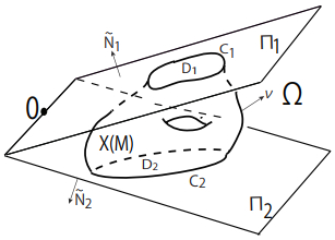
We study a variational problem for hypersurfaces in a wedge in the Euclidean space. Our wedge is bounded by a finitely many hyperplanes passing a common point. The total energy of each hypersurface is the sum of its anisotropic surface energy and the wetting energy of the planar domain bounded by the boundary of the considered hypersurface. An anisotropic surface energy is a generalization of the surface area which was introduced to model the surface tension of a small crystal. We show an existence and uniqueness result of local minimizers of the total energy among hypersurfaces enclosing the same volume. Our result is new even when the special case where the surface energy is the surface area.
Citation: Miyuki Koiso. Stable anisotropic capillary hypersurfaces in a wedge[J]. Mathematics in Engineering, 2023, 5(2): 1-22. doi: 10.3934/mine.2023029
We study a variational problem for hypersurfaces in a wedge in the Euclidean space. Our wedge is bounded by a finitely many hyperplanes passing a common point. The total energy of each hypersurface is the sum of its anisotropic surface energy and the wetting energy of the planar domain bounded by the boundary of the considered hypersurface. An anisotropic surface energy is a generalization of the surface area which was introduced to model the surface tension of a small crystal. We show an existence and uniqueness result of local minimizers of the total energy among hypersurfaces enclosing the same volume. Our result is new even when the special case where the surface energy is the surface area.

| [1] |
N. Ando, Hartman-Wintner's theorem and its applications, Calc. Var., 43 (2012), 389–402. http://doi.org/10.1007/s00526-011-0415-x doi: 10.1007/s00526-011-0415-x

|
| [2] |
J. L. Barbosa, M. Do Carmo, J. Eschenburg, Stability of hypersurfaces of constant mean curvature in Riemannian manifolds, Math. Z., 197 (1988), 123–138. https://doi.org/10.1007/BF01161634 doi: 10.1007/BF01161634
|
| [3] |
J. Choe, M. Koiso, Stable capillary hypersurfaces in a wedge, Pac. J. Math., 280 (2016), 1–15. http://doi.org/10.2140/pjm.2016.280.1 doi: 10.2140/pjm.2016.280.1
|
| [4] |
Y. He, H. Li, Integral formula of Minkowski type and new characterization of the Wulff shape, Acta. Math. Sin.-English Ser., 24 (2008), 697–704. https://doi.org/10.1007/s10114-007-7116-6 doi: 10.1007/s10114-007-7116-6
|
| [5] |
Y. He, H. Li, H. Ma, J. Ge, Compact embedded hypersurfaces with constant higher order anisotropic mean curvatures, Indiana Univ. Math. J., 58 (2009), 853–868. http://doi.org/10.1512/iumj.2009.58.3515 doi: 10.1512/iumj.2009.58.3515
|
| [6] | M. Koiso, Uniqueness of stable closed non-smooth hypersurfaces with constant anisotropic mean curvature, arXiv.1903.03951. |
| [7] |
M. Koiso, Uniqueness of closed equilibrium hypersurfaces for anisotropic surface energy and application to a capillary problem, Math. Comput. Appl., 24 (2019), 88. https://doi.org/10.3390/mca24040088 doi: 10.3390/mca24040088
|
| [8] |
M. Koiso, B. Palmer, Geometry and stability of surfaces with constant anisotropic mean curvature, Indiana Univ. Math. J., 54 (2005), 1817–1852. http://doi.org/10.1512/iumj.2005.54.2613 doi: 10.1512/iumj.2005.54.2613
|
| [9] |
M. Koiso, B. Palmer, Stability of anisotropic capillary surfaces between two parallel planes, Calc. Var., 25 (2006), 275–298. http://doi.org/10.1007/s00526-005-0336-7 doi: 10.1007/s00526-005-0336-7
|
| [10] |
M. Koiso, B. Palmer, Anisotropic capillary surfaces with wetting energy, Calc. Var., 29 (2007), 295–345. http://doi.org/10.1007/s00526-006-0066-5 doi: 10.1007/s00526-006-0066-5
|
| [11] |
M. Koiso, B. Palmer, Uniqueness theorems for stable anisotropic capillary surfaces, SIAM J. Math. Anal., 39 (2007), 721–741. https://doi.org/10.1137/060657297 doi: 10.1137/060657297
|
| [12] |
M. Koiso, B. Palmer, Anisotropic umbilic points and Hopf's theorem for surfaces with constant anisotropic mean curvature, Indiana Univ. Math. J., 59 (2010), 79–90. http://doi.org/10.1512/iumj.2010.59.4164 doi: 10.1512/iumj.2010.59.4164
|
| [13] |
H. Li, C. Xiong, Stability of capillary hypersurfaces with planar boundaries, J. Geom. Anal., 27 (2017), 79–94. https://doi.org/10.1007/s12220-015-9674-7 doi: 10.1007/s12220-015-9674-7
|
| [14] |
B. Palmer, Stability of the Wulff shape, Proc. Am. Math. Soc., 126 (1998), 3661–3667. http://doi.org/10.1090/S0002-9939-98-04641-3 doi: 10.1090/S0002-9939-98-04641-3
|
| [15] |
R. C. Reilly, The relative differential geometry of nonparametric hypersurfaces, Duke Math. J., 43 (1976), 705–721. http://doi.org/10.1215/S0012-7094-76-04355-6 doi: 10.1215/S0012-7094-76-04355-6
|
| [16] | R. Schneider, Convex bodies: the Brunn-Minkowski theory, 2 Eds., New York: Cambridge University Press, 2014. https://doi.org/10.1017/CBO9781139003858 |
| [17] |
J. E. Taylor, Crystalline variational problems, Bull. Amer. Math. Soc., 84 (1978), 568–588. https://doi.org/10.1090/S0002-9904-1978-14499-1 doi: 10.1090/S0002-9904-1978-14499-1
|
| [18] |
H. Weyl, On the volume of tubes, Amer. J. Math., 61 (1939), 461–472. https://doi.org/10.2307/2371513 doi: 10.2307/2371513
|
| [19] |
W. L. Winterbottom, Equilibrium shape of a small particle in contact with a foreign substrate, Acta Metal., 15 (1967), 303–310. https://doi.org/10.1016/0001-6160(67)90206-4 doi: 10.1016/0001-6160(67)90206-4
|
| [20] |
G. Wulff, Zur Frage der Geschwindigkeit des Wachsthums und der Auflösung der Krystallflächen, Zeitschrift für Krystallographie und Mineralogie, 34 (1901), 449–530. https://doi.org/10.1524/zkri.1901.34.1.449 doi: 10.1524/zkri.1901.34.1.449
|

Figures(2)

Miyuki Koiso. Stable anisotropic capillary hypersurfaces in a wedge[J]. Mathematics in Engineering, 2023, 5(2): 1-22. doi: 10.3934/mine.2023029


 DownLoad: