A multi-layer reactive transport model for fractured porous media

Luca Formaggia; Alessio Fumagalli; Anna Scotti; Luca Formaggia; Alessio Fumagalli; Anna Scotti

doi:10.3934/mine.2022008

Mathematics in Engineering

2022, Volume 4, Issue 1: 1-32. doi: 10.3934/mine.2022008

Previous Article Next Article

Research article Special Issues

A multi-layer reactive transport model for fractured porous media

Dipartimento di Matematica, Politecnico di Milano, piazza Leonardo da Vinci 32, 20133 Milano, Italy

Received: 06 November 2020 Accepted: 18 May 2021 Published: 10 June 2021

An accurate modeling of reactive flows in fractured porous media is a key ingredient to obtain reliable numerical simulations of several industrial and environmental applications. For some values of the physical parameters we can observe the formation of a narrow region or layer around the fractures where chemical reactions are focused. Here, the transported solute may precipitate and form a salt, or vice-versa. This phenomenon has been observed and reported in real outcrops. By changing its physical properties, this layer might substantially alter the global flow response of the system and thus the actual transport of solute: the problem is thus non-linear and fully coupled. The aim of this work is to propose a new mathematical model for reactive flow in fractured porous media, by approximating both the fracture and these surrounding layers via a reduced model. In particular, our main goal is to describe the layer thickness evolution with a new mathematical model, and compare it to a fully resolved equidimensional model for validation. As concerns numerical approximation we extend an operator splitting scheme in time to solve sequentially, at each time step, each physical process thus avoiding the need for a non-linear monolithic solver, which might be challenging due to the non-smoothness of the reaction rate. We consider bi- and tridimensional numerical test cases to asses the accuracy and benefit of the proposed model in realistic scenarios.
- fractured porous media,
- reactive flow in porous media,
- mixed-dimensional modeling,
- reduced order modeling,
- operator splitting
Citation: Luca Formaggia, Alessio Fumagalli, Anna Scotti. A multi-layer reactive transport model for fractured porous media[J]. Mathematics in Engineering, 2022, 4(1): 1-32. doi: 10.3934/mine.2022008

Related Papers:

Abstract

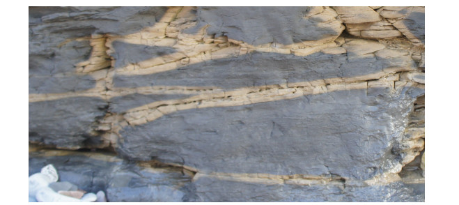
An accurate modeling of reactive flows in fractured porous media is a key ingredient to obtain reliable numerical simulations of several industrial and environmental applications. For some values of the physical parameters we can observe the formation of a narrow region or layer around the fractures where chemical reactions are focused. Here, the transported solute may precipitate and form a salt, or vice-versa. This phenomenon has been observed and reported in real outcrops. By changing its physical properties, this layer might substantially alter the global flow response of the system and thus the actual transport of solute: the problem is thus non-linear and fully coupled. The aim of this work is to propose a new mathematical model for reactive flow in fractured porous media, by approximating both the fracture and these surrounding layers via a reduced model. In particular, our main goal is to describe the layer thickness evolution with a new mathematical model, and compare it to a fully resolved equidimensional model for validation. As concerns numerical approximation we extend an operator splitting scheme in time to solve sequentially, at each time step, each physical process thus avoiding the need for a non-linear monolithic solver, which might be challenging due to the non-smoothness of the reaction rate. We consider bi- and tridimensional numerical test cases to asses the accuracy and benefit of the proposed model in realistic scenarios.

References

[1]	J. Aghili, K. Brenner, J. Hennicker, R. Masson, L. Trenty, Two-phase discrete fracture matrix models with linear and nonlinear transmission conditions, Int. J. Geomath., 10 (2019), 1. doi: 10.1007/s13137-019-0118-6
[2]	A. Agosti, L. Formaggia, A. Scotti, Analysis of a model for precipitation and dissolution coupled with a darcy flux, J. Math. Anal. Appl., 431 (2015), 752-781. doi: 10.1016/j.jmaa.2015.06.003
[3]	A. Agosti, B. Giovanardi, L. Formaggia, A. Scotti, A numerical procedure for geochemical compaction in the presence of discontinuous reactions, Adv. Water Resour., 94 (2016), 332-344. doi: 10.1016/j.advwatres.2016.06.001
[4]	P. F. Antonietti, C. Facciolà, A. Russo, M. Verani, Discontinuous Galerkin approximation of flows in fractured porous media on polytopic grids, SIAM J. Sci. Comput., 41 (2019), A109-A138. doi: 10.1137/17M1138194
[5]	P. F. Antonietti, L. Formaggia, A. Scotti, M. Verani, N. Verzotti, Mimetic finite difference approximation of flows in fractured porous media, ESAIM: M2AN, 50 (2016), 809-832. doi: 10.1051/m2an/2015087
[6]	J. Bear, A. H. D. Cheng, Modeling groundwater flow and contaminant transport, Springer, 2010.
[7]	I. Berre, W. M. Boon, B. Flemisch, A. Fumagalli, D. Gläser, E. Keilegavlen, et al., Verification benchmarks for single-phase flow in three-dimensional fractured porous media, Adv. Water Resour., 147 (2021), 103759. doi: 10.1016/j.advwatres.2020.103759
[8]	D. Boffi, F. Brezzi, M. Fortin, Mixed finite element methods and applications, Berlin, Heidelberg: Springer, 2013.
[9]	W. M. Boon, J. M. Nordbotten, I. Yotov, Robust discretization of flow in fractured porous media, SIAM J. Numer. Anal., 56 (2018), 2203-2233. doi: 10.1137/17M1139102
[10]	W. M. Boon, J. M. Nordbotten, J. E. Vatne, Functional analysis and exterior calculus on mixed-dimensional geometries, Annali di Matematica, 200 (2021), 757-789. doi: 10.1007/s10231-020-01013-1
[11]	N. Bouillard, R. Eymard, R. Herbin, P. Montarnal, Diffusion with dissolution and precipitation in a porous medium: Mathematical analysis and numerical approximation of a simplified model, ESAIM: M2AN, 41 (2007), 975-1000. doi: 10.1051/m2an:2007047
[12]	K. Brenner, J. Hennicker, R. Masson, P. Samier, Hybrid-dimensional modelling of two-phase flow through fractured porous media with enhanced matrix fracture transmission conditions, J. Comput. Phys., 357 (2018), 100-124. doi: 10.1016/j.jcp.2017.12.003
[13]	K. Brenner, M. Groza, C. Guichard, R. Masson, Vertex approximate gradient scheme for hybrid dimensional two-phase darcy flows in fractured porous media, ESAIM: M2AN, 49 (2015), 303-330. doi: 10.1051/m2an/2014034
[14]	C. Bringedal, L. von Wolff, I. S. Pop, Phase field modeling of precipitation and dissolution processes in porous media: Upscaling and numerical experiments, Multiscale Model. Sim., 18 (2020), 1076-1112. doi: 10.1137/19M1239003
[15]	F. Chave, D. A. Di Pietro, L. Formaggia, A hybrid high-order method for darcy flows in fractured porous media, SIAM J. Sci. Comput., 40 (2018), A1063-A1094. doi: 10.1137/17M1119500
[16]	I. Faille, A. Fumagalli, J. Jaffré, J. E. Roberts, Model reduction and discretization using hybrid finite volumes of flow in porous media containing faults, Comput. Geosci., 20 (2016), 317-339. doi: 10.1007/s10596-016-9558-3
[17]	E. Flauraud, F. Nataf, I. Faille, R. Masson, Domain decomposition for an asymptotic geological fault modeling, CR Mècanique, 331 (2003), 849-855.
[18]	B. Flemisch, I. Berre, W. Boon, A. Fumagalli, N. Schwenck, A. Scotti, et al., Benchmarks for single-phase flow in fractured porous media, Adv. Water Resour., 111 (2018), 239-258. doi: 10.1016/j.advwatres.2017.10.036
[19]	B. Flemisch, H. Rainer, Numerical investigation of a mimetic finite difference method, In: Finite volumes for complex applications V - problems and perspectives, Wiley - VCH, 2018,815-824.
[20]	L. Formaggia, A. Fumagalli, A. Scotti, P. Ruffo, A reduced model for Darcy's problem in networks of fractures, ESAIM: M2AN, 48 (2014), 1089-1116. doi: 10.1051/m2an/2013132
[21]	L. Formaggia, A. Scotti, F. Sottocasa, Analysis of a mimetic finite difference approximation of flows in fractured porous media, ESAIM: M2AN, 52 (2018), 595-630. doi: 10.1051/m2an/2017028
[22]	A. Fumagalli, I. Faille, A double-layer reduced model for fault flow on slipping domains with hybrid finite volume scheme, SIAM J. Sci. Comput., 77 (2018), 1-26. doi: 10.1007/s10915-018-0692-z
[23]	A. Fumagalli, E. Keilegavlen, S. Scialò, Conforming, non-conforming and non-matching discretization couplings in discrete fracture network simulations, J. Comput. Phys., 376 (2019), 694-712. doi: 10.1016/j.jcp.2018.09.048
[24]	A. Fumagalli, L. Pasquale, S. Zonca, S. Micheletti, An upscaling procedure for fractured reservoirs with embedded grids, Water Resour. Res., 52 (2016), 6506-6525. doi: 10.1002/2015WR017729
[25]	A. Fumagalli, A. Scotti, A numerical method for two-phase flow in fractured porous media with non-matching grids, Adv. Water Resour., 62 (2013), 454-464. doi: 10.1016/j.advwatres.2013.04.001
[26]	A. Fumagalli, A. Scotti, A multi-layer reduced model for flow in porous media with a fault and surrounding damage zones, Comput. Geosci., 24 (2020), 1347-1360. doi: 10.1007/s10596-020-09954-5
[27]	A. Fumagalli, A. Scotti, Reactive flow in fractured porous media, In: Finite volumes for complex applications IX - methods, theoretical aspects, examples, Cham: Springer International Publishing, 2020, 55-73.
[28]	A. Fumagalli, A, Scotti, A mathematical model for thermal single-phase flow and reactive transport in fractured porous media, J. Comput. Phys., 434 (2021), 110205. doi: 10.1016/j.jcp.2021.110205
[29]	B. Giovanardi, A. Scotti, L. Formaggia, P. Ruffo, A general framework for the simulation of geochemical compaction, Comput. Geosci., 19 (2015), 1027-1046. doi: 10.1007/s10596-015-9518-3
[30]	E. Keilegavlen, R. Berge, A. Fumagalli, M. Starnoni, I. Stefansson, J. Varela, et al., Porepy: An open-source software for simulation of multiphysics processes in fractured porous media, Comput. Geosci., 25, (2021), 243-265.
[31]	P. Knabner, C. J. van Duijn, S. Hengst, An analysis of crystal dissolution fronts in flows through porous media. part 1: Compatible boundary conditions, Adv. Water Resour., 18 (1995), 171-185. doi: 10.1016/0309-1708(95)00005-4
[32]	T. V. Lopes, A. C. Rocha, M. A. Murad, E. L. M. Garcia, P. A. Pereira1, C. L. Cazarin, A new computational model for flow in karst-carbonates containing solution-collapse breccias, Comput. Geosci., 24 (2020), 61-87. doi: 10.1007/s10596-019-09894-9
[33]	V. Martin, J. Jaffré, J. E. Roberts, Modeling fractures and barriers as interfaces for flow in {P}orous media, SIAM J. Sci. Comput., 26 (2005), 1667-1691. doi: 10.1137/S1064827503429363
[34]	J. M. Nordbotten, W. Boon, A. Fumagalli, E. Keilegavlen, Unified approach to discretization of flow in fractured porous media, Comput. Geosci., 23 (2019), 225-237. doi: 10.1007/s10596-018-9778-9
[35]	I. S. Pop, J. Bogers, K. Kumar, Analysis and upscaling of a reactive transport model in fractured porous media with nonlinear transmission condition, Vietnam J. Math., 45 (2017), 77-102. doi: 10.1007/s10013-016-0198-7
[36]	F. A. Radu, I. S. Pop, S. Attinger, Analysis of an Euler implicit - mixed finite element scheme for reactive solute transport in porous media, Numer. Meth. PDE, 26 (2010), 320-344.
[37]	P. A. Raviart, J. M. Thomas, A mixed finite element method for second order elliptic problems, In: Mathematical aspects of finite element methods, Berlin, Heidelberg: Springer, 1977,292-315.
[38]	J. E. Roberts, J. M. Thomas, Mixed and hybrid methods, In: Handbook of numerical analysis, Vol. II, Amsterdam: North-Holland, 1991,523-639.
[39]	N. Schwenck, B. Flemisch, R. Helmig, B. Wohlmuth, Dimensionally reduced flow models in fractured porous media: crossings and boundaries, Comput. Geosci., 19 (2015), 1219-1230. doi: 10.1007/s10596-015-9536-1
[40]	I. Stefansson, I. Berre, E. Keilegavlen, Finite-volume discretisations for flow in fractured porous media, Transport Porous Med., 124 (2018), 439-462. doi: 10.1007/s11242-018-1077-3
[41]	M. Tene, S. B. M. Bosma, M. S. Al Kobaisi, H. Hajibeygi, Projection-based embedded discrete fracture model (pEDFM), Adv. Water Resour., 105 (2017), 205-216. doi: 10.1016/j.advwatres.2017.05.009
[42]	T. L. van Noorden, Crystal precipitation and dissolution in a porous medium: effective equations and numerical experiments, Multiscale Model. Sim., 7 (2009), 1220-1236. doi: 10.1137/080722096

Reader Comments

Your name:*

Email:*
© 2022 the Author(s), licensee AIMS Press. This is an open access article distributed under the terms of the Creative Commons Attribution License (http://creativecommons.org/licenses/by/4.0)