Endophytes colonizing plant tissue play an essential role in plant growth, development, stress tolerance and plant protection from soil-borne diseases. In this study, we report the diversity of cultivable endophytic bacteria associated with marigold (Calendula officinalis L.) by using 16S rRNA gene analysis and their plant beneficial properties. A total of 42 bacterial isolates were obtained from plant tissues of marigold. They belonged to the genera Pantoea, Enterobacter, Pseudomonas, Achromobacter, Xanthomonas, Rathayibacter, Agrobacterium, Pseudoxanthomonas, and Beijerinckia. Among the bacterial strains, P. kilonensis FRT12, and P. rhizosphaerae FST5 showed moderate or vigorous inhibition against three tested plant pathogenic fungi, F. culmorum, F. solani and R. solani. They also demonstrated the capability to produce hydrolytic enzymes and indole-3-acetic acid (IAA). Five out of 16 isolates significantly stimulated shoot and root growth of marigold in a pot experiment. The present study reveals that more than half of the bacterial isolates associated with marigold (C. officinalis L.) provided antifungal activity against one or more plant pathogenic fungi. Our findings suggest that medicinal plants with antimicrobial activity could be a source for selecting microbes with antagonistic activity against fungal plant pathogens or with plant growth stimulating potential. These isolates might be considered as promising candidates for the improvement of plant health.
Citation: Vyacheslav Shurigin, Burak Alaylar, Kakhramon Davranov, Stephan Wirth, Sonoko Dorothea Bellingrath-Kimura, Dilfuza Egamberdieva. Diversity and biological activity of culturable endophytic bacteria associated with marigold (Calendula officinalis L.)[J]. AIMS Microbiology, 2021, 7(3): 336-353. doi: 10.3934/microbiol.2021021
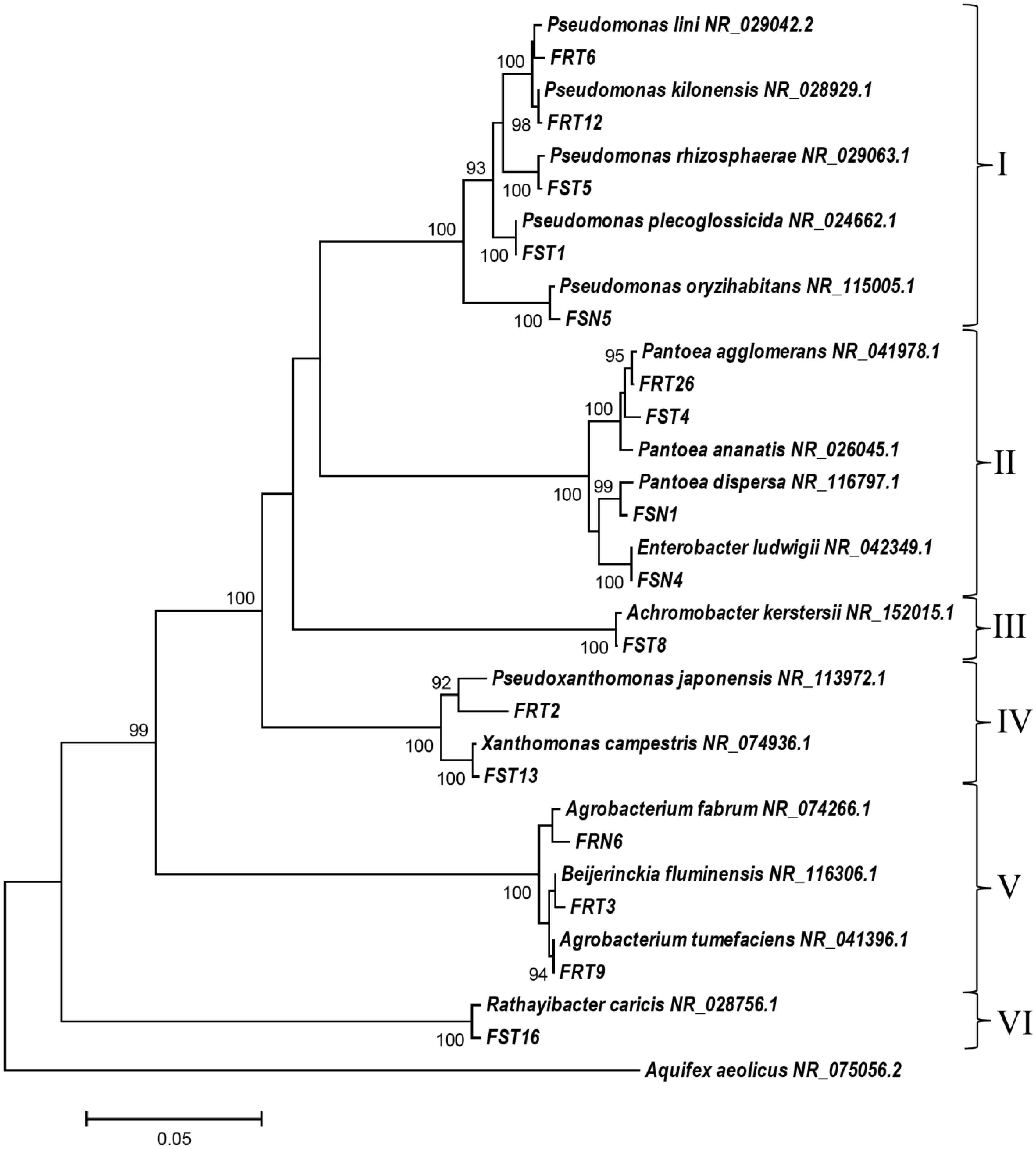
Endophytes colonizing plant tissue play an essential role in plant growth, development, stress tolerance and plant protection from soil-borne diseases. In this study, we report the diversity of cultivable endophytic bacteria associated with marigold (Calendula officinalis L.) by using 16S rRNA gene analysis and their plant beneficial properties. A total of 42 bacterial isolates were obtained from plant tissues of marigold. They belonged to the genera Pantoea, Enterobacter, Pseudomonas, Achromobacter, Xanthomonas, Rathayibacter, Agrobacterium, Pseudoxanthomonas, and Beijerinckia. Among the bacterial strains, P. kilonensis FRT12, and P. rhizosphaerae FST5 showed moderate or vigorous inhibition against three tested plant pathogenic fungi, F. culmorum, F. solani and R. solani. They also demonstrated the capability to produce hydrolytic enzymes and indole-3-acetic acid (IAA). Five out of 16 isolates significantly stimulated shoot and root growth of marigold in a pot experiment. The present study reveals that more than half of the bacterial isolates associated with marigold (C. officinalis L.) provided antifungal activity against one or more plant pathogenic fungi. Our findings suggest that medicinal plants with antimicrobial activity could be a source for selecting microbes with antagonistic activity against fungal plant pathogens or with plant growth stimulating potential. These isolates might be considered as promising candidates for the improvement of plant health.

| [1] |
Danielski L, Campos LMAS, Bresciani LFV, et al. (2007) Marigold (Calendula officinalis L.) oleoresin: Solubility in SC-CO2 and composition profile. Chem Eng Prog 46: 99-106. doi: 10.1016/j.cep.2006.05.004

|
| [2] | Jan N, Andrabi KI, John R (2017) Calendula officinalis-an important medicinal plant with potential biological properties. Proc Indian Natn Sci Acad 83: 769-787. |
| [3] | Verma PK, Raina R, Agarwal S, et al. (2018) Phytochemical ingredients and pharmacological potential of Calendula officinalis Linn. Pharm Biomed Res 4: 1-17. |
| [4] | Chakraborty GS (2010) Phytochemical screening of Calendula officinalis Linn leaf extract by TLC. Int J Res Ayurveda Pharm 1: 131-134. |
| [5] |
Shapour HCh, Mehrdad AK, Abdollah GP (2016) Phytochemical analysis and antibacterial effects of Calendula officinalis essential oil. Biosci Biotech Res Comm 9: 517-522. doi: 10.21786/bbrc/9.3/26
|
| [6] | Shankar ShM, Bardvalli SG, Jyotirmayee R, et al. (2017) Efficacy of Calendula officinalis extract (marigold flower) as an antimicrobial agent against oral microbes: an in vitro study in comparison with chlorhexidine digluconate. J Clin Diagn Res 11: ZC05-ZC10. |
| [7] |
Cromack HTH, Smith JM (1998) Calendula officinalis-production potential and crop agronomy in southern England. Ind Crop Prod 7: 223-229. doi: 10.1016/S0926-6690(97)00052-6
|
| [8] | Abdel-Wahed GA (2020) Application of some fungicides alternatives for management root rot and wilt fungal diseases of marigold (Calendula officinalis L.). Sci J Agric Sci 2: 31-41. |
| [9] | Sohi HS (1983) Personal communication on disease of marigold Banglore: IIHR. |
| [10] | Singh VK, Singh Y, Kumar P (2012) Diseases of ornamental plants and their management. Eco-friendly innovative approaches in plant disease management New Delhi: International Book Distributors and Publisher, 543-572. |
| [11] | Pirone PP (1978) Diseases and pests of ornamental plants Chichester: John Wiley and Sons. |
| [12] | Bharnwal MK, Jha DK, Dubey SC (2002) Evaluation of fungicides against Alternaria blight of marigold (Tagetes sp.). J Res BAU 14: 99-100. |
| [13] | Kumar V (2012) Marigold diseases and its control. Agropedia Available from: http://agropedia.iitk.ac.in/content/marigold-diseases-its-control. |
| [14] | Szwejkowska B, Bielski S (2012) Effect of nitrogen and magnesium fertilization on the development and yields of pot marigold (Calendula officinalis L.). Acta Sci Pol Hortorum Cultus 11: 141-148. |
| [15] | Hussein MM, Sakr RA, Badr LA, et al. (2011) Effect of some fertilizers on botanical and chemical characteristics of pot marigold plant (Calendula officinalis L.). J Hortic Sci Ornament Plants 3: 220-231. |
| [16] |
Krol B (2011) The effect of different nitrogen fertilization rates on yield and quality of marigold (Calendula officinalis L. ‘Tokaj’) raw material. Acta Agrobot 64: 29-34. doi: 10.5586/aa.2011.027
|
| [17] |
Banchio E, Bogino P, Zygadlo J, et al. (2008) Plant growth promoting rhizobacteria improve growth and essential oil yield in Origanum majorana L. Biochem Syst Ecol 36: 766-771. doi: 10.1016/j.bse.2008.08.006
|
| [18] |
Egamberdieva D, Li L, Lindström K, et al. (2015a) A synergistic interaction between salt tolerant Pseudomonas and Mezorhizobium strains improves growth and symbiotic performance of liquorice (Glycyrrhiza uralensis Fish.) under salt stress. Appl Microbiol Biotechnol 100: 2829-2841. doi: 10.1007/s00253-015-7147-3
|
| [19] |
Egamberdieva D, Shurigin V, Gopalakrishnan S, et al. (2015b) Microbial strategies for the improvement of legume production in hostile environments. Legumes under environmental stress: yield, improvement and adaptations UK: John Wiley & Sons Ltd, 133-144. doi: 10.1002/9781118917091.ch9
|
| [20] |
White JF, Kingsley KL, Zhang Q, et al. (2019) Review: Endophytic microbes and their potential applications in crop management. Pest Manag Sci 75: 2558-2565. doi: 10.1002/ps.5527
|
| [21] | Egamberdieva D, Kamilova F, Validov S, et al. (2008) High incidence of plant growth-stimulating bacteria associated with the rhizosphere of wheat grown in salinated soil in Uzbekistan. Environ Microbiol 19: 1-9. |
| [22] |
Egamberdieva D, Kucharova Z, Davranov K, et al. (2011) Bacteria able to control foot and root rot and to promote growth of cucumber in salinated soils. Biol Fertil Soils 47: 197-205. doi: 10.1007/s00374-010-0523-3
|
| [23] |
Pawlik M, Cania B, Thijs S, et al. (2017) Hydrocarbon degradation potential and plant growth-promoting activity of culturable endophytic bacteria of Lotus corniculatus and Oenothera biennis from a long-term polluted site. Environ Sci Pollut Res 24: 19640-19652. doi: 10.1007/s11356-017-9496-1
|
| [24] |
Koberl M, Ramadan EM, Adam M, et al. (2013) Bacillus and Streptomyces were selected as broad-spectrum antagonists against soilborne pathogens from arid areas in Egypt. FEMS Microbiol Lett 342: 168-178. doi: 10.1111/1574-6968.12089
|
| [25] |
Dodd IC, Zinovkina NY, Safronova VI, et al. (2010) Rhizobacterial mediation of plant hormone status. Ann Appl Biol 157: 361-379. doi: 10.1111/j.1744-7348.2010.00439.x
|
| [26] |
Egamberdieva D, Wirth S, Alqarawi AA, et al. (2017a) Phytohormones and beneficial microbes: Essential components for plants to balance stress and fitness. Front Microbiol 8: 2104. doi: 10.3389/fmicb.2017.02104
|
| [27] |
Shurigin V, Egamberdieva D, Li L, et al. (2020a) Endophytic bacteria associated with halophyte Seidlitzia rosmarinus Ehrenb. ex Boiss. from arid land of Uzbekistan and their plant beneficial traits. J Arid Land 12: 730-740. doi: 10.1007/s40333-020-0019-4
|
| [28] |
Glick BR (2014) Bacteria with ACC deaminase can promote plant growth and help to feed the world. Microbiol Res 169: 30-39. doi: 10.1016/j.micres.2013.09.009
|
| [29] |
Shurigin V, Egamberdieva D, Samadiy S, et al. (2020b) Endophytes from medicinal plants as biocontrol agents against fusarium caused diseases. Mikrobiol Z 82: 41-52. doi: 10.15407/microbiolj82.04.041
|
| [30] |
Alemu F (2016) Isolation of Pseudomonas flurescens from rhizosphere of faba bean and screen their hydrogen cyanide production under in vitro study, Ethiopia. Am J Life Sci 4: 13-19. doi: 10.11648/j.ajls.20160402.11
|
| [31] | Hashem A, Abd_Allah EF, Alqarawi A, et al. (2016) The interaction between arbuscular mycorrhizal fungi and endophytic bacteria enhances plant growth of Acacia gerrardii under salt stress. Front Plant Sci 7: 1089. |
| [32] |
Chung EJ, Hossain MT, Khan A, et al. (2015) Bacillus oryzicola sp. Nov., an endophytic bacterium isolated from the roots of rice with antimicrobial, plant growth promoting, and systemic resistance inducing activities in rice. Plant Pathol J 31: 152-164. doi: 10.5423/PPJ.OA.12.2014.0136
|
| [33] | Mao JN, Zhang XY, Gong MF (2016) Disease resistance induction in rice by inoculation with endophytic bacteria strain REB01. ICESSD 2015 459-464. |
| [34] |
Hastuti US, Al-Asna PM, Rahmawati D (2018) Histologic observation, identification, and secondary metabolites analysis of endophytic fungi isolated from a medicinal plant, Hedichium acuminatum Roscoe. AIP Conf Proc 2002: 020070Available from: https://doi.org/10.1063/1.5050166. doi: 10.1063/1.5050166
|
| [35] |
Salam N, Khieu TN, Liu MJ, et al. (2017) Endophytic actinobacteria associated with Dracaena cochinchinensis Lour.: isolation, diversity, and their cytotoxic activities. Biomed Res Int 2017: 1308563. doi: 10.1155/2017/1308563
|
| [36] |
Egamberdieva D, Shurigin V, Alaylar B, et al. (2020b) Bacterial endophytes from horseradish (Armoracia rusticana G. Gaertn., B. Mey. & Scherb.) with antimicrobial efficacy against pathogens. Plant Soil Environ 66: 309-316. doi: 10.17221/137/2020-PSE
|
| [37] |
Ait Kaki A, Kacem Chaouche N, Dehimat L, et al. (2013) Biocontrol and plant growth promotion characterization of Bacillus species isolated from Calendula officinalis rhizosphere. Indian J Microbiol 53: 447-452. doi: 10.1007/s12088-013-0395-y
|
| [38] |
Katoch M, Pull S (2017) Endophytic fungi associated with Monarda citriodora, an aromatic and medicinal plant and their biocontrol potential. Pharm Biol 55: 1528-1535. doi: 10.1080/13880209.2017.1309054
|
| [39] | Mohammadi AM, Ebrahimi A, Mahzonieh MR, et al. (2021) Antibacterial activities of bacterial endophytes isolated from Zataria multiflora, Achillea willhelmsii and Calendula officinalis L against some human nosocomial pathogens. Zahedan J Res Med Sci 18: e2482. |
| [40] | Dashti AA, Jadaon MM, Abdulsamad AM, et al. (2009) Heat treatment of bacteria: a simple method of DNA extraction for molecular techniques. Kuwait Med J 41: 117-122. |
| [41] | Lane DJ (1991) 16S/23S rRNA Sequencing. Nucleic Acid Techniques in Bacterial Systematic New York: John Wiley and Sons, 115-175. |
| [42] | Jinneman KC, Wetherington JH, Adams AM, et al. (1996) Differentiation of Cyclospora sp. and Eimeria spp. by using the polymerase chain reaction amplification products and restriction fragment length polymorphisms. FDA Lab Information Bulletin LIB 4044: Available from: http://vm.cfsan.fda.gov/~mow/kjcsl9c.html. |
| [43] | Saitou N, Nei M (1987) The neighbor-joining method: a new method for reconstructing phylogenetic trees. Mol Biol Evol 4: 406-425. |
| [44] |
Felsenstein J (1985) Confidence limits on phylogenies: An approach using the bootstrap. Evolution 39: 783-791. doi: 10.1111/j.1558-5646.1985.tb00420.x
|
| [45] |
Tamura K, Nei M, Kumar S (2004) Prospects for inferring very large phylogenies by using the neighbor-joining method. Proc Natl Acad Sci USA 101: 11030-11035. doi: 10.1073/pnas.0404206101
|
| [46] |
Tamura K, Stecher G, Peterson D (2013) MEGA6: molecular evolutionary genetics analysis version 6.0. Mol Biol Evol 30: 2725-2729. doi: 10.1093/molbev/mst197
|
| [47] |
Elissawy AM, Ebada SS, Ashour ML, et al. (2019) New secondary metabolites from the mangrove-derived fungus Aspergillus sp. AV-2. Phytochem Lett 29: 1-5. doi: 10.1016/j.phytol.2018.10.014
|
| [48] |
Rojsanga P, Gritsanapan W, Suntornsuk L (2006) Determination of berberine content in the stem extracts of Coscinium fenestratum by TLC densitometry. Med Princ Pract 15: 373-378. doi: 10.1159/000094272
|
| [49] |
Bano N, Musarrat J (2003) Characterization of a new Pseudomonas aeruginosa strain NJ-15 as a potential biocontrol agent. Curr Microb 46: 324-328. doi: 10.1007/s00284-002-3857-8
|
| [50] |
Castric PA (1975) Hydrogen cyanide, a secondary metabolite of Pseudomonas aeruginosa. Can J Microbiol 21: 613-618. doi: 10.1139/m75-088
|
| [51] |
Lugtenberg BJJ, Kravchenko LV, Simons M (1999) Tomato seed and root exudate sugars: composition, utilization by Pseudomonas biocontrol strains and role in rhizosphere colonization. Environ Microbiol 1: 439-446. doi: 10.1046/j.1462-2920.1999.00054.x
|
| [52] |
Walsh GA, Murphy RA, Killeen GF, et al. (1995) Technical note: detection and quantification of supplemental fungal beta-glucanase activity in animal feed. J Anim Sci 73: 1074-1076. doi: 10.2527/1995.7341074x
|
| [53] |
Brown MRW, Foster JHS (1970) A simple diagnostic milk medium for Pseudomonas aeruginosa. J Clin Pathol 23: 172-177. doi: 10.1136/jcp.23.2.172
|
| [54] | Malleswari D, Bagyanarayan G (2013) In vitro screening of rhizobacteria isolated from the rhizosphere of medicinal and aromatic plants for multiple plant growth promoting activities. J Microbiol Biotechnol Res 3: 84-91. |
| [55] |
Howe TG, Ward JM (1976) The utilization of tween 80 as carbon source by Pseudomonas. J Gen Microbiol 92: 234-235. doi: 10.1099/00221287-92-1-234
|
| [56] |
Egamberdieva D, Kucharova Z (2009) Selection for root colonising bacteria stimulating wheat growth in saline soils. Biol Fertil Soils 45: 561-573. doi: 10.1007/s00374-009-0366-y
|
| [57] |
Mohamad OA, Li L, Ma JB, et al. (2018) Evaluation of the antimicrobial activity of endophytic bacterial populations from Chinese traditional medicinal plant licorice and characterization of the bioactive secondary metabolites produced by Bacillus atrophaeus against Verticillium dahliae. Front Microbiol 9: 924. doi: 10.3389/fmicb.2018.00924
|
| [58] |
Akinsanya MA, Goh JKh, Lim SP, et al. (2015) Diversity, antimicrobial and antioxidant activities of culturable bacterial endophyte communities in Aloe vera. FEMS Microbiol Lett 362: fnv184. doi: 10.1093/femsle/fnv184
|
| [59] |
Uche-Okereafor N, Sebola T, Tapfuma K, et al. (2019) Antibacterial activities of crude secondary metabolite extracts from Pantoea species obtained from the stem of Solanum mauritianum and their effects on two cancer cell lines. Int J Environ Res Public Health 16: 602. doi: 10.3390/ijerph16040602
|
| [60] |
Bulgarelli D, Schlaeppi K, Spaepen S, et al. (2013) Structure and functions of the bacterial microbiota of plants. Annu Rev Plant Biol 64: 807-838. doi: 10.1146/annurev-arplant-050312-120106
|
| [61] |
Chi F, Shen S, Cheng H, et al. (2005) Ascending migration of endophytic rhizobia, from roots to leaves, inside rice plants and assessment of benefits to rice growth physiology. Appl Environ Microbiol 71: 7271-7278. doi: 10.1128/AEM.71.11.7271-7278.2005
|
| [62] | Egamberdieva D, Wirth S, Behrendt U, et al. (2017c) Antimicrobial activity of medicinal plants correlates with the proportion of antagonistic endophytes. Front Microbiol 8: 199. |
| [63] |
Shurigin V, Davranov K, Wirth S, et al. (2018) Medicinal plants with phytotoxic activity harbour endophytic bacteria with plant growth inhibitory properties. Environ Sustainability 1: 209-215. doi: 10.1007/s42398-018-0020-4
|
| [64] | Goryluk A, Rekosz-Burlaga H, Blaszczyk M (2009) Isolation and characterization of bacterial endophytes of Chelidonium majus L. Pol J Microbiol 58: 355-361. |
| [65] |
Egamberdieva D, Wirth S, Li L (2017b) Microbial cooperation in the rhizosphere improves liquorice growth under salt stress. Bioengineered 8: 433-438. doi: 10.1080/21655979.2016.1250983
|
| [66] |
Mehanni MM, Safwat MS (2010) Endophytes of medicinal plants. Acta Hortic 854: 31-40. doi: 10.17660/ActaHortic.2010.854.3
|
| [67] |
Nongkhlaw FMW, Joshi SR (2014) Epiphytic and endophytic bacteria that promote growth of ethnomedicinal plants in the subtropical forests of Meghalaya, India. Rev Biol Trop 62: 1295-1308. doi: 10.15517/rbt.v62i4.12138
|
| [68] |
Egamberdieva D, Wirth SJ, Shurigin VV, et al. (2017d) Endophytic bacteria improve plant growth, symbiotic performance of chickpea (Cicer arietinum L.) and induce suppression of root rot caused by Fusarium solani under salt stress. Front Microbiol 8: 1887. doi: 10.3389/fmicb.2017.01887
|
| [69] |
Liu Y, Mohamad OAA, Salam N, et al. (2019) Diversity, community distribution and growth promotion activities of endophytes associated with halophyte Lycium ruthenicum Murr. 3 Biotech 9: 144. doi: 10.1007/s13205-019-1678-8
|
| [70] |
Egamberdieva D, Shurigin V, Alaylar B, et al. (2020a) The effect of biochars and endophytic bacteria on growth and root rot disease incidence of Fusarium infested narrow-leafed lupin (Lupinus angustifolius L.). Microorganisms 8: 496. doi: 10.3390/microorganisms8040496
|
| [71] |
Ferchichi N, Toukabri W, Boularess M, et al. (2019) Isolation, identification and plant growth promotion ability of endophytic bacteria associated with lupine root nodule grown in Tunisian soil. Arch Microbiol 201: 1333-1349. doi: 10.1007/s00203-019-01702-3
|
| [72] | Fernando TC, Cruz JA (2019) Profiling and biochemical ıdentification of potential plant growth-promoting endophytic bacteria from Nypa fruticans. Philipp J Crop Sci 44: 77-85. |
| [73] | Rana KL, Kour D, Yadav AH (2019) Endophytic microbiomes: Biodiversity, ecological significance and biotechnological applications. Res J Biotechnol 14: 142-162. |
| [74] | Siddiqui ZA (2005) PGPR: prospective biocontrol agents of plant pathogens. PGPR: biocontrol and biofertilization Dordrecht: Springer, 111-142. |
| [75] |
Michelsen CF, Stougaard P (2012) Hydrogen cyanide synthesis and antifungal activity of the biocontrol strain Pseudomonas fluorescens In5 from Greenland is highly dependent on growth medium. Can J Microbiol 58: 381-390. doi: 10.1139/w2012-004
|
| [76] |
Ahmed EA, Hassan EA, El Tobgy KMK, et al. (2014) Evaluation of rhizobacteria of some medicinal plants for plant growth promotion and biological control. Ann Agric Sci 59: 273-280. doi: 10.1016/j.aoas.2014.11.016
|
| [77] |
Musa Z, Ma J, Egamberdieva D, et al. (2020) Diversity and antimicrobial potential of cultivable endophytic actinobacteria associated with medicinal plant Thymus roseus. Front Microbiol 11: 191. doi: 10.3389/fmicb.2020.00191
|
| [78] | Hemavathi VN, Sivakumr BS, Suresh CK, et al. (2006) Effect of Glomus fasciculatum and Plant Growth Promoting Rhizobacteria on growth and yield of Ocimum basilicum. Karnataka J Agric Sci 19: 17-20. |
| [79] | Hosseinzadah F, Satei A, Ramezanpour MR (2011) Effects of mycorrhiza and plant growth promoting rhizobacteria on growth, nutrient uptake and physiological characteristics in Calendula officinalis L. Middle East J Sci Res 8: 947-953. |
| [80] | Karthikeyan B, Joe MM, Jaleel CA, et al. (2010) Effect of root inoculation with plant growth promoting rhizobacteria (PGPR) on plant growth, alkaloid content and nutrient control of Catharanthus roseus (L.) G. Don. Nat Croat 19: 205-212. |
| [81] |
Rahmoune B, Morsli A, Khelifi-Slaoui M, et al. (2017) Isolation and characterization of three new PGPR and their effects on the growth of Arabidopsis and Datura plants. J Plant Interact 12: 1-6. doi: 10.1080/17429145.2016.1269215
|
| [82] |
Egamberdieva D, Berg G, Lindstrom K, et al. (2010) Co-inoculation of Pseudomonas spp. with Rhizobium improves growth and symbiotic performance of fodder galega (Galega orientalis Lam.). Eur J Soil Biol 46: 269-272. doi: 10.1016/j.ejsobi.2010.01.005
|
| [83] |
Rasool A, Mir MI, Zulfajri M, et al. (2021) Plant growth promoting and antifungal asset of indigenous rhizobacteria secluded from saffron (Crocus sativus L.) rhizosphere. Microb Pathog 150: 104734. doi: 10.1016/j.micpath.2021.104734
|
 microbiol-07-03-021-s001.pdf microbiol-07-03-021-s001.pdf |
 |
Figures(1) / Tables(4)

Vyacheslav Shurigin, Burak Alaylar, Kakhramon Davranov, Stephan Wirth, Sonoko Dorothea Bellingrath-Kimura, Dilfuza Egamberdieva. Diversity and biological activity of culturable endophytic bacteria associated with marigold (Calendula officinalis L.)[J]. AIMS Microbiology, 2021, 7(3): 336-353. doi: 10.3934/microbiol.2021021


 DownLoad: