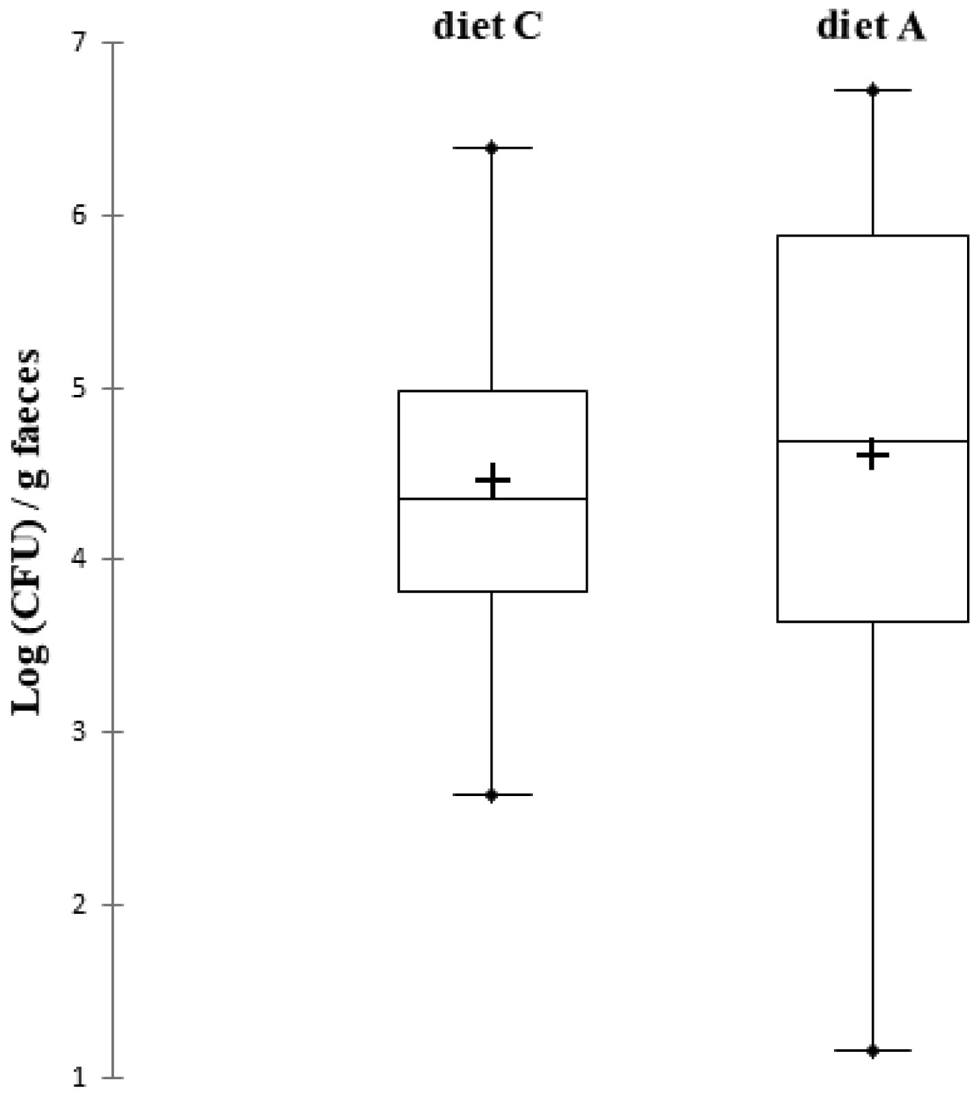
Cranberry (<i>Vaccinium macrocarpon</i>) dietary supplementation and fecal microbiota of Wistar rats

Rayane Chettaoui; Gilles Mayot; Loris De Almeida; Patrick Di Martino; Rayane Chettaoui; Gilles Mayot; Loris De Almeida; Patrick Di Martino

doi:10.3934/microbiol.2021016

AIMS Microbiology

2021, Volume 7, Issue 2: 257-270. doi: 10.3934/microbiol.2021016

Previous Article Next Article

Research article Special Issues

Cranberry (Vaccinium macrocarpon) dietary supplementation and fecal microbiota of Wistar rats

Laboratoire ERRMECe, CY Cergy Paris University, 1 rue Descartes 95000 Neuville-sur-Oise, France

Received: 06 May 2021 Accepted: 29 June 2021 Published: 30 June 2021

Cranberry (Vaccinium macrocarpon) dietary supplementation can help prevention of urinary tract infections through the supply of proanthocyanidin-type polyphenols (PAC). The main uropathogenic bacteria are members of the intestinal microbiota. A randomized cross-over experiment was done to investigate whether cranberry dietary supplementation affects concentrations of thermotolerant coliforms, Enterococcus spp. and Lactobacillus spp. in rat faeces. Thirteen rats, housed in individual cages, received successively two diets as pellets during 7 days each: a standard diet without polyphenols and the standard diet supplemented with cranberry powder containing 10.9 mg/100 g of PAC. There was a 7 days wash-out period in between with standard diet without polyphenols. Body weight and feed intake were recorded. Faeces were collected on the last day of treatment, and crushed to count the different bacterial populations using the most probable number method. Thermotolerant coliforms were grown in BGBLB tubes and on MacConkey agar. Enterococcus spp. were grown in Rothe and Litsky broths and on KF Streptococcus agar. Lactobacillus spp. were grown in Man Rogosa Sharpe broth. Body mass gains were not affected by cranberry supplementation. This is consistent with equal food intake, cranberry powder not providing significant energy supplement. Cranberry dietary supplementation was associated with changes in fecal concentrations of thermotolerant coliforms, and Enterococcus spp. in some rats, but did not induce significant changes in bacterial fecal concentrations in a global population of 13 rats. In conclusion, we did not observe any significant effect of dietary cranberry supplementation on the fecal microbiota of Wistars rats for a 7-day diet.

Keywords:

Citation: Rayane Chettaoui, Gilles Mayot, Loris De Almeida, Patrick Di Martino. Cranberry (Vaccinium macrocarpon) dietary supplementation and fecal microbiota of Wistar rats[J]. AIMS Microbiology, 2021, 7(2): 257-270. doi: 10.3934/microbiol.2021016

Related Papers:

[1]	J. A. López Molina, M. J. Rivera, E. Berjano . Electrical-thermal analytical modeling of monopolar RF thermal ablation of biological tissues: determining the circumstances under which tissue temperature reaches a steady state. Mathematical Biosciences and Engineering, 2016, 13(2): 281-301. doi: 10.3934/mbe.2015003
[2]	Hu Dong, Gang Liu, Xin Tong . Influence of temperature-dependent acoustic and thermal parameters and nonlinear harmonics on the prediction of thermal lesion under HIFU ablation. Mathematical Biosciences and Engineering, 2021, 18(2): 1340-1351. doi: 10.3934/mbe.2021070
[3]	Andriy A. Avramenko, Igor V. Shevchuk . Renormalization group analysis of heat transfer in the presence of endothermic and exothermic chemical reactions. Mathematical Biosciences and Engineering, 2019, 16(4): 2049-2062. doi: 10.3934/mbe.2019100
[4]	Abdulaziz Alsenafi, M. Ferdows . Effects of thermal slip and chemical reaction on free convective nanofluid from a horizontal plate embedded in a porous media. Mathematical Biosciences and Engineering, 2021, 18(4): 4817-4833. doi: 10.3934/mbe.2021245
[5]	P. Vafeas, A. Skarlatos, P. K. Papadopoulos, P. Svarnas, N. Sarmas . A boundary value problem of heat transfer within DBD-based plasma jet setups. Mathematical Biosciences and Engineering, 2023, 20(10): 18345-18367. doi: 10.3934/mbe.2023815
[6]	EYK Ng, Leonard Jun Cong Looi . Numerical analysis of biothermal-fluids and cardiac thermal pulse of abdominal aortic aneurysm. Mathematical Biosciences and Engineering, 2022, 19(10): 10213-10251. doi: 10.3934/mbe.2022479
[7]	Weirui Lei, Jiwen Hu, Yatao Liu, Wenyi Liu, Xuekun Chen . Numerical evaluation of high-intensity focused ultrasound- induced thermal lesions in atherosclerotic plaques. Mathematical Biosciences and Engineering, 2021, 18(2): 1154-1168. doi: 10.3934/mbe.2021062
[8]	Hafiz Muhammad Muzzammil, Yong-De Zhang, Hassan Ejaz, Qihang Yuan, Muhammad Muddassir . A review on tissue-needle interaction and path planning models for bevel tip type flexible needle minimal intervention. Mathematical Biosciences and Engineering, 2024, 21(1): 523-561. doi: 10.3934/mbe.2024023
[9]	Aamir Saeed, Rehan Ali Shah, Muhammad Sohail Khan, Unai Fernandez-Gamiz, Mutasem Z. Bani-Fwaz, Samad Noeiaghdam, Ahmed M. Galal . Theoretical analysis of unsteady squeezing nanofluid flow with physical properties. Mathematical Biosciences and Engineering, 2022, 19(10): 10176-10191. doi: 10.3934/mbe.2022477
[10]	Rui Zhang, Shuicai Wu, Weiwei Wu, Hongjian Gao, Zhuhuang Zhou . Computer-assisted needle trajectory planning and mathematical modeling for liver tumor thermal ablation: A review. Mathematical Biosciences and Engineering, 2019, 16(5): 4846-4872. doi: 10.3934/mbe.2019244

Abstract

Nomenclature

$x$ : coordinate measure in axial direction (m)

$r$ : coordinate measure in radial direction (m)

$u$ : velocity component along axial direction (ms $^{-1}$ )

$v$ : velocity component along radial direction (ms $^{-1}$ )

$u_w$ : velocity of the moving needle (ms $^{-1}$ )

$u_\infty$ : velocity outside the boundary layer (ms $^{-1}$ )

$u_c$ : composite velocity (ms $^{-1}$ )

$T$ : temperature of fluid (K)

$T_w$ : wall temperature (K)

$T_\infty$ : ambient temperature (K)

$K(T)$ : thermal conductivity (m $^2$ s $^{-1}$ )

$\mu(T)$ : dynamic viscosity (kgm $^{-1}$ s $^{-1}$ )

$\rho_f$ : density of fluid (kgm $^{-3}$ )

$C_b$ : drag coefficient (Jkg $^{-1}$ K $^{-1}$ )

$\sigma_s$ : Boltzman constant (Wm $^{-2}$ K $^{-4}$ )

$\rho C_p$ : effective heat capacitance (Jm $^{-3}$ K $^{-1}$ )

$\psi$ : stream function (m $^{2}$ s $^{-1}$ )

$\upsilon_f$ : kinematic viscosity (m $^{2}$ s $^{-1}$

$\chi$ : needle size

$B_0$ : applied magnetic field

$k^*$ : permeability of porous medium

$k_e$ : mean absorption coefficient

$M$ : magnetic parameter

$k_1$ : porosity parameter

$Rd$ : radiation parameter

$\hbar$ : convergence control parameter

$F_r$ : inertia parameter

$\epsilon$ : velocity ratio parameter

$\delta_k$ : thermal conductivity parameter

$\delta_\mu$ : variable viscosity parameter

$Re$ : Reynolds number

$Ec$ : Eckert number

$Pr$ : Prandtl number

$\mathscr{L}$ : auxiliary linear operator

1. Introduction

There is the transmission of heat from a solid body to a gas or liquid flow in a problem whose consideration involves the science of fluid motion. A flow of heat is layered on the physical motion of a fluid, and the two fields interact. In order to obtain the temperature distribution and the heat transfer rate, it is important to connect the equation of motion with the energy conservation equation. However, a comprehensive solution for the flow of a viscous fluid around a body involves significant mathematical difficulties for all fluid flow geometries. To overcome such difficulties, in the year 1904 the German aerodynamicist Ludwig Prandtl ^[1] introduced the concept of a boundary layer. The boundary layer idea fills a gap between the theories and practices that had previously existed (for one thing, it introduces the theoretical possibilities of drag). Furthermore, the boundary layer approach allowed the solution of viscous flow problems that would have been difficult to solve through the application of the Navier-Stokes equation to the entire flow field. Prandtl ^[1] showed that several viscous flow problems may be investigated by splitting them into two areas, one near solid boundaries and the other spanning the rest of the flow. Only in the thin region near a solid boundary (the boundary layers) is the influence of viscosity important. The influence of viscosity is insignificant in the region outside of the boundary layers and the fluid can be viewed as non-viscous.

Heat transfer analysis and Darcy-Forchheimer flow in porous media are utilized in a wide range of applications. Porous media can be naturally formed (e.g., wood, sponges, sand beds, rocks) or fabricated (e.g., wicks, insulation, catalytic pellet). Schaefer ^[2] provided an overview of engineered porous materials, while Shafer et al. ^[3] covered the chemistry and physics of porous media. Bilal et al. ^[4] investigated the convective Casson fluid flow with homogeneous‒heterogeneous reactions in a Darcy-Forchheimer medium. The analysis of heat transfer and entropy generation in a stratified MHD (magnetohydrodynamic) Carreau nanofluid with gyrotactic microorganisms was performed by Naz et al. ^[5]. They also studied the thermal and species transportation of Eyring-Powell material over a rotating disk with swimming microorganisms ^[6]. A numerical investigation of Darcy-Forchheimer and EMHD nanofluid flow toward a porous medium was performed by Rasool et al. ^[7]. Flow of porous media can find extensive industrial and scientific uses in numerous natural settings such as geothermal energy systems, hydrology, petroleum reservoirs, crude gas and oil productions, granular insulation, catalytic reactors, water movements in reservoirs, grain storage, fermentation processes and so on (see, for example, Das et al. ^[8], Dogonchi et al. ^[9], Ajarostagi ^[10] and Abdelmalek et al. ^[11]).

Heat transfer and boundary layer flow across a thin needle has become a topic of interest in current studies because of their significant applications in hot-wire anemometers, biomedicine, extrusion of a plastic sheet, wire coating, continuous casting, submarines, geothermal power generation, lubrication and the cooling of electronic devices. The thin needle is considered as a body of revolution with a thickness that is less than the thickness of the boundary layer. Lee ^[12] initially considered the boundary layer formation adjacent to a thin needle in a viscous fluid. Chen and Smith ^[13] investigated the analytical solution of a steady forced convective laminar flow across a non-isothermal thin needle. Grosan and Pop ^[14] used the bvp4c programming in MATLAB software to investigate the forced convective flow across a thin needle in a nanofluid. The mixed convective boundary layer flow across vertically moving thin needles was explored by Wang ^[15] who calculated the numerical solution for assisting and opposing flow and discovered that the solution for assisting flow is unique, but the solution for opposing flow may be unique, dual or non-existent. The formation of boundary layer flow across a non-isothermal needle which moves in a parallel free stream, has been studied in the work ^[16] in which the Keller box approach was used to calculate the numerical solution to discover that dual solutions occur when a needle moves in the reverse direction of the free stream. The mixed convective flow of a water base and ethylene glycol nanofluid across a non-isothermal thin needle was investigated by Nayak et al. ^[17] by using a generalized differential quadrature approach. They discovered that the copper ethylene glycol based nanofluid shows the greatest improvement in the heat transfer rate. The effect of Lorentz forces and Darcy-Forchheimer on radiative nanofluid flow toward a slippery curved geometry was analyzed by Algehyne et al. ^[18]. A collection of the boundary layer flow across a thin needle with different physical effect in nanofluid can be seen in the works by Hayat et al. ^[19], Ahmad et al. ^[20], Narain and Uberoi ^[21], Ahmad et al. ^[22], Afridi et al. ^[23] and Sulochana et al. ^[24,25].

The investigation of exchanges of thermal flow of a fluid through different objects has attracted researchers because of its essential physical applications including air flow past an aircraft and wind engineering. Moreover, thermal radiation is also used in different fields of technology, including biomedicine, space equipment, drilling processes, cancer treatment, and higher temperature procedures. Nadeem et al. ^[26] investigated the influence of thermal radiation on the boundary layer flow of a Jeffrey fluid across an exponential stretch surface by using the homotopy analysis method (HAM) to solve the problem analytically. The effects of chemical reactions and thermal radiation on MHD nanofluid have been investigated by Arulmozhi et al. ^[27]. In the presence of thermal radiation and a heat source/sink, a steady boundary layer flow of Powell-Eyring nanofluid toward a stretching sheet was numerically explored by Manvi et al. ^[28]. Tayebi et al. ^[29] performed numerical analysis for thermal natural convection as well as the entropy generation of (Al $_2$ O $_3$ -H $_2$ O) nanoparticles toward a circular cylinder. Chamkha et al. ^[30] investigated the natural convection MHD nanofluid in a cavity with a radiation effect and shape factor of nanoparticles. Seyyedi et al. ^[31] examined the natural convection heat transfer and entropy generation for hexagonal cavities with a magnetic field and (Cu-H $_2$ O) nanoliquid. Dogonchi et al. ^[32] studied MHD nanofluid flow in parallel disks during a suction/blowing process with radiation and viscous dissipation effects. Wakif ^[33] investigated a steady 2D MHD convective flow of a radiative Casson fluid toward a horizontal stretching sheet. Sandeep et al. ^[34] investigated the effect of nonlinear thermal radiation on MHD hybrid nanofluid flow with a heat source. Salleh et al. ^[35] investigated the impact of a magnetic field across a vertically moving thin needle in nanofluid. With MHD radiative nanofluid and stability analysis, the researchers in ^[36] examined the boundary layer flow and heat transmission rate through a traveling thin needle. Khan et al. ^[37] investigated magnetohydrodynamic thin film flow through a porous stretching sheet by focusing on the impact of thermal radiation and viscous dissipation. Jawad et al. ^[38] discussed the analysis of hybrid nanofluid stagnation point flow over a stretching surface by focusing on melting heat transfer. Ramzan et al. ^[39] investigated the effect of melting heat transfer on the flow across a moving needle with a magnetic field. Kumar and Upreti ^[40] described the MHD nanofluid flow across a thin needle by employing the Joule heating effect. The researchers in ^[41] explored two-dimensional (2D) forced convective MHD nanofluid flow across a horizontally traveling thin needle with viscous dissipation and a heat source or sinks. Hamid ^[42] used chemical reactions and nonlinear thermal radiation to study the MHD Casson nanofluid flow along a vertically positioned thin needle. The impact of the Darcy-Forchheimer flow for visco-elastic fluid across a thin needle was explored by Raju et al. ^[43]. Using viscous dissipation, the researchers in ^[44] investigated the formation of entropy for hybrid nanofluid flow across a needle. Nazar et al. ^[45] explored the hybrid nanofluid flow of Au-TiO $_2$ nanoparticles across a thin needle in the presence of thermal radiation and magnetic field effects with duality solution and stability analysis. The rate of heat transfer on the MHD Casson nanofluid toward a thin needle embedded in a porous medium with non-linear radiation effects was explored by Akinshilo et al. ^[46]. The researchers in ^[47] studied dynamic control by applying the HAM for nonlinear shallow water wave equations. Based on the stochastic arithmetic, Noeiaghdam et al. ^[48] found optimal convergence control parameters in the HAM for integral equations. In another work ^[49], the authors combined the HAM with Laplace transform method to produce a new powerful method named the homotopy analysis transform method. They also combined the HAM with Wazwaz's regularization method to produce the homotopy regularization method for solving integral equations (see ^[50]).

It is well known that perturbation and asymptotic approximations of nonlinear problems are often broken down as nonlinearity becomes strong. Therefore, they are only valid for weakly nonlinear ODEs and PDEs in general. The HAM is an analytic approximation method for highly nonlinear problems; unlike perturbation techniques, the HAM is independent of any small/large physical parameters at all. Second, different from all of the other analytic techniques, the HAM provides us a convenient way to guarantee the convergence of the solution series so that it is valid even if nonlinearity becomes rather strong. Besides, based on the homotopy of topology, it provides us much freedom to choose the base functions, initial guesses and so on, so that complicated nonlinear ODEs and PDEs can often be solved in a simple way.

In summary, the HAM has the following advantages and disadvantages:

● Independent of small/large physical parameters.

● Guarantee of convergence.

● Flexibility on choice of base function and initial guess.

● Great generality.

● It can always provide analytic approximation efficiently, but it does not give an exact solution.

● More convergence control parameters might give better approximation, but it needs much more CPU time.

There are many publications dealing with heat transfer relating to nanofluid flow across a thin needle in the above-mentioned and other related literature, but there is hardly any study of 2D boundary layer MHD nanofluid flow across a horizontally moving thin needle with nonlinear thermal radiation. Therefore, the current study aims to fill this gap. The novelty of this work is the study of the effects of thermal radiation, a magnetic field, variable viscosity parameters, temperature ratio parameter and thermal conductivity parameters on the MHD boundary layer flow of a nanofluid across a porous thin needle. To studies these effects we dissolved titanium dioxide (TiO $_2$ ) in water to make (TiO $_2$ -H $_2$ O) nanofluid. In the presence of viscous dissipation, the governing PDEs are described and are then transformed into a system of nonlinear ODEs by using an appropriate similarity transformation. The HAM algorithm is utilized to determine the solution of the modeled equations. To ensure that our code is proper, we conducted a comparison study with several earlier findings. The study presented here possesses step implementation in several engineering and industrial processes and is provides responses to the following questions below:

$1)$ How does the rate of heat transfer improve with the addition of titanium dioxide (TiO $_2$ ) in the base fluid water?

$2)$ What is the behavior of the velocity and temperature profiles against the decreasing size of the needle?

$3)$ What is the behavior of the velocity and temperature profiles against the varying values of variable viscosity and thermal conductivity parameters, respectively?

2. Physical description and mathematical modeling

In this section, we will present our problem in both physical and mathematical forms. Initially the problem will be explained physically through a schematic diagram and then the obtained physical descriptions will be modeled mathematically. The main physical quantities of this study are discussed in the next subsection. Throughout this phenomenon, some relevant parameters will be encountered that will be defined mathematically with a physical explanation in the conclusion part of this section.

2.1. Physical description of the problem

We consider a steady 2D boundary layer MHD nanofluid flow across a thin needle with nonlinear thermal radiation. The thin needle flow is also considered to be laminar and viscous. The needle is considered to be moving horizontally with uniform velocity $u_w$ in a uniform stream velocity $u_{\infty}$ as illustrated in . We assume that $v(x, r)$ and $u(x, r)$ are the components of the velocity along the radial and axial directions, respectively. The constant wall temperature at the thin needle surface and their corresponding ambient temperature are respectively, denoted by $T_w$ and $T_{\infty}$ , where $T_{\infty} < T_w$ . For the given flow system, the radius of a thin needle is defined by

$\begin{equation} \begin{array}{l} r = R(x) = \sqrt{\frac{\chi\upsilon x}{u_c}}, \end{array} \end{equation}$

(2.1)

Figure 1. Geometry of the flow problem.

DownLoad: Full-Size Img PowerPoint

where $\chi$ represent the needle size and $u_c = u_w+u_{\infty}$ is the composite velocity. With a low Reynolds number assumption (see ^[51]), a magnetic field with magnetic intensity $B_0$ is applied, which eventually results in the induced magnetic field being ignored. We further assume that the size of the needle is thin as compared to the boundary layer thickness that forms over it, so that the pressure gradient of the needle is neglected, while the impact of curvature in the transverse direction cannot be ignored.

2.2. Mathematical modeling of the problem

Keeping in view all of the assumptions described in subsection (2.1), the governing boundary layer equation of the nanofluid flow problem transforms as follows (see ^[52] and ^[53]):

$\begin{equation} \begin{array}{l} \frac{\partial}{\partial x}(ru)+\frac{\partial}{\partial r}(rv) = 0, \end{array} \end{equation}$

(2.2)

$\begin{equation} \begin{array}{l} u\frac{\partial u}{\partial x}+v\frac{\partial v}{\partial r} = \frac{\mu(T)}{\rho_{f}}\left[\frac{1}{r}\frac{\partial u}{\partial r}+\frac{\partial^2 u}{\partial r^2}\right]+\frac{1}{\rho_f}\frac{\partial u}{\partial r}\frac{\partial \mu(T)}{\partial T}-\frac{\upsilon_f}{k^*}u-\frac{C_b}{\rho_f\sqrt{k^*}}u^2-\frac{\sigma B^2_0}{\rho_f}u, \end{array} \end{equation}$

(2.3)

and

$\begin{equation} \begin{array}{l} & u\frac{\partial T}{\partial x}+v\frac{\partial T}{\partial r} = \frac{K(T)}{\rho C_p}\left[\frac{1}{r}\frac{\partial}{\partial r}\left(r\frac{\partial T}{\partial r}\right)-\frac{16\sigma_sT^3_{\infty}}{3K(T)k_e}\frac{1}{r}\frac{\partial}{\partial r}\left(r\frac{\partial T}{\partial r}\right)\right]+\frac{1}{\rho C_p}\left(\frac{\partial T}{\partial r}\right)^2\frac{\partial K(T)}{\partial T}+\\ &\frac{\mu(T)}{\rho C_p}\left(\frac{\partial u}{\partial r}\right)^2+\frac{\sigma B^2_0}{\rho C_p}u^2, \end{array} \end{equation}$

(2.4)

subjected to the physical boundary conditions (BCs) given by

$\begin{equation} \begin{array}{l} u = u_w, \quad v = 0, \quad T = T_w, \quad at \quad r = R(x) \quad and \quad u\to u_{\infty}, \quad T\to T_{\infty} \quad as \quad r\to \infty. \end{array} \end{equation}$

(2.5)

The thermal conductivity and kinematic viscosity of the nanofluid are respectively, denoted by $K(T)$ and $\mu(T)$ and are defined as follows (see ^[54]):

$\begin{equation} \begin{array}{l} K(T) = K_0\left[1+\delta_k\frac{T-T_{\infty}}{T_w-T_{\infty}}\right], \quad \mu(T) = \frac{\rho\upsilon_f}{1+\delta_\mu(T-T_{\infty})}. \end{array} \end{equation}$

(2.6)

In Eqs (2.2) to (2.6), the velocity components in the radial and axial directions are given, respectively, by $v$ and $u$ . Here $\rho$ , $u_w$ , $C_p$ , $T$ , $T_w$ , $T_{\infty}$ , $k^*$ , $C_b$ , $B_0$ , $u_{\infty}$ , $\delta_{\mu}$ and $\delta_k$ represent the density, velocity of the moving needle, specific heat, temperature, constant surface temperature, ambient temperature, permeability of porous medium, drag coefficient, applied magnetic field, velocity outside the boundary layer, variable viscosity and thermal conductivity parameter.

To convert the model described by Eqs (2.2) to (2.4) with the BCs in Eq (2.5), we shall use the following set of similarity variables (see ^[55]):

$\begin{equation} \begin{array}{l} \eta = \frac{u_cr^2}{\upsilon x}, \quad \psi = \upsilon xF(\eta), \quad \Theta = \frac{T-T_{\infty}}{T_w-T_{\infty}}. \end{array} \end{equation}$

(2.7)

After applying the Rosseland approximation, the heat flux is simplified as follows:

$\begin{equation} \begin{array}{l} q_r = -\frac{4\sigma_s}{3k_e}\frac{\partial T^4}{\partial r}, \end{array} \end{equation}$

(2.8)

where $\sigma_s$ is the Boltzman constant and $k_e$ is the mean absorption coefficient. Expanding $T_{\infty}$ by means of the Taylor series and neglecting the higher-order terms, the preceding equation can be expressed in the following form:

$\begin{equation} \begin{array}{l} q_r = -\frac{16\sigma_s}{3k_e}T^3_{\infty}\frac{\partial T}{\partial r}. \end{array} \end{equation}$

(2.9)

The present study is streamlined, so $\psi$ represents a stream function in Eq (2.7). Thus the flow characteristic component for the proposed stream function are as follows:

$\begin{equation} \begin{array}{l} u = \frac{1}{r}\frac{\partial \psi}{\partial r}, \quad v = -\frac{1}{r}\frac{\partial \psi}{\partial x}. \end{array} \end{equation}$

(2.10)

After incorporating Eqs (2.7) and (2.10) with the relation given by Eq (2.6) into Eqs (2.2) to (2.4), we obtain the following sets of ODEs after some simplification:

$\begin{equation} \begin{array}{l} \left[\frac{2\eta}{1+\delta_\mu\Theta}\right]F^{\prime\prime\prime}+\frac{1}{1+\delta_\mu\Theta}(F^{\prime\prime}-2\eta F^{\prime\prime}\Theta)-\frac{1}{2}(M+k_1)F^{\prime}-F_rF^{\prime}+\eta F^{\prime}F^{\prime\prime}+FF^{\prime\prime} = 0, \end{array} \end{equation}$

(2.11)

$\begin{equation} \begin{array}{l} \frac{1+\delta_{k}\Theta}{Pr}\left[1+\frac{4Rd}{3(1+\delta_{k}\Theta)}\left(((1+\theta_{r})\Theta^3)(\eta\Theta^{\prime})\right)^{\prime}\right]+2\eta\Theta^{\prime}F^{\prime}+2\Theta^{\prime}F+\frac{4}{Pr}(1+\delta_{k}\Theta)\eta\Theta^{\prime^2}\\+16EcF^{\prime\prime^2}+MEcF^{\prime^2} = 0. \end{array} \end{equation}$

(2.12)

The dimensionless form of the subjected BCs are given by

$\begin{equation} \begin{array}{l} F(\eta) = \frac{\chi\epsilon}{2}, \quad \Theta(\eta) = 1, \quad F^{\prime}(\eta) = \frac{\epsilon}{2} \quad at \quad \eta = \chi, \\ F^{\prime}(\eta)\to \frac{1-\epsilon}{2}, \quad \Theta(\eta)\to 0 \quad as \quad \eta\to\infty. \end{array} \end{equation}$

(2.13)

It should be noticed that the parameter $\epsilon = \frac{u_w}{u_c}$ represents a significant characteristic for the flow system which is described as (a) when $\epsilon = 0$ , then the needle is static and the fluid is moving; (b) when $\epsilon = 1$ , then the needle is moving and the fluid is static; (c) when $0 < \epsilon < 1$ , then the fluid and the needle are moving in the same directions. Furthermore, in Eqs (2.11) to (2.13) we have various emerging parameters which are present in Table 1 along with the mathematical description and physical interpretation of each of them.

Table 1. Information of physical parameters.

Symbolic notations	Mathematical description	Physical interpretation
$M$	$\frac{\sigma B^2_0x}{\rho_fu_c}$	Magnetic parameter
$k_1$	$\frac{\upsilon_fx}{k^*u_c}$	Porosity parameter
$Rd$	$\frac{4\sigma_sT^3_{\infty}}{k_e}$	Radiation parameter
$F_r$	$\frac{C_bx}{\sqrt{k^*}\rho_fu_c}$	Inertia parameter
$\epsilon$	$\frac{u_w}{u_c}$	Velocity ratio parameter
$\theta_r$	$\frac{T_w}{T_{\infty}}$	Temperature ratio parameter
$\delta_\mu$	$\delta^*_{\mu}(T_w-T_{\infty})$	Variable viscosity parameter
$Pr$	$\frac{\rho C_p\upsilon_f}{K_0}$	Prandtl number
$Re$	$\frac{xu_c}{\upsilon_f}$	Reynolds number
$Ec$	$\frac{{u_c}^2}{C_p(T_w-T_{\infty})}$	Eckert number

| Show Table

DownLoad: CSV

2.3. Skin friction and Nusselt number

The skin friction coefficient and the local Nusselt number for our flow system are expressed as follows:

$\begin{equation} \begin{array}{l} \left.C_f = \frac{2\mu(T)}{\rho(u_c)^2}u_r\right|_{r = \chi}, \quad \left.Nu = \frac{-xT_r}{T_w-T_{\infty}}+q_r\right|_{r = \chi}. \end{array} \end{equation}$

(2.14)

Using Eq (2.7) in Eq (2.14), we have these physical quantities in dimensionless form as given below (see ^[56]):

$\begin{equation} \begin{array}{l} \left.{\rm Re}^{\frac{1}{2}}C_f = \frac{8\sqrt{\chi}}{1+\delta_{\mu}}F_{\eta\eta}\right|_{\eta = \chi}, \quad \left.{\rm Re}^{-\frac{1}{2}}Nu = -2\sqrt{\chi}\left(1+\frac{4}{3(1+\delta_k\Theta)}Rd\right)\left(((\theta_r-1)\Theta\right)^3\Theta_{\eta})\right|_{\eta = \chi}. \end{array} \end{equation}$

(2.15)

Here ${\rm Re} = \frac{xu_c}{\upsilon_f}$ denotes the Reynolds number.

3. Main idea of HAM

It is well known that nonlinear ODEs and PDEs for boundary value problems are much more difficult to solve than linear ODEs and PDEs, especially by means of analytic methods. Traditionally, perturbation and asymptotic techniques are widely applied to obtain analytic approximations of nonlinear problems in science, finance and engineering. Unfortunately, perturbation and asymptotic techniques are too strongly dependent upon small/large physical parameters in general, and thus are often valid only for weakly nonlinear problems. Thus, it is necessary to develop some analytic approximation methods, which are independent of any small/large physical parameters at all and valid for strongly nonlinear problems. Therefore, in 1992, one of such kind of analytic approximation methods was proposed by the author of ^[58], namely the HAM.

First of all, based on the homotopy of topology, the HAM is independent of any small/large physical parameters at all. So, unlike asymptotic/perturbation techniques, the HAM can be applied to solve most nonlinear problems in science, finance and engineering, especially those without small/large physical parameters. Second, unlike all other analytical techniques, the HAM provides us a convenient way to guarantee the convergence of the solution series so that it is valid for highly nonlinear problems. Third, the HAM provides us much freedom to choose the auxiliary linear operator and base functions. Using such kind of freedom, some complicated nonlinear problems can be solved in a much easier way. Finally, the HAM logically contains the Lyapunov small artificial parameter method, Adomian decomposition method, the $\delta$ -expansion method and the Euler transform. Thus, it has great generality.

Let us first consider a nonlinear differential equation

$\begin{equation} \begin{array}{l} \mathscr{N}[u(x, t)] = 0, \end{array} \end{equation}$

(3.1)

where $\mathscr{N}$ is a nonlinear operator, $x$ is a vector of all spatial independent variables, $t$ denotes the temporal independent variable and $u(x, t)$ is an unknown function, Liao ^[58] constructed a two-parameter family of equations in the embedding parameter $q\in$ [0, 1], called the zeroth-order deformation equation

$\begin{equation} \begin{array}{l} (1-q)\mathscr{L}[\phi(x, t;q)-u_0(x, t)] = \hbar q\mathscr{N}[\phi(x, t;q)], \end{array} \end{equation}$

(3.2)

where $\mathscr{L}$ is an auxiliary linear operator, $\hbar$ is a non-zero auxiliary parameter, $\phi(x, t; q)$ is an unknown function and $u_0(x)$ is an initial guess. At $q$ = 0 and $q$ = 1 we have

$\begin{equation} \begin{array}{l} \phi(x, t;0) = u_0(x, t), \end{array} \end{equation}$

(3.3)

$\begin{equation} \begin{array}{l} \phi(x, t;1) = u(x, t). \end{array} \end{equation}$

(3.4)

As the embedding parameter $q\in$ [0, 1] increases from 0 to 1, the solution $\phi(x, t; q)$ of the zeroth-order deformation equation deforms from the initial guess $u_0(x, t)$ to the exact solution $u(x, t)$ of the original nonlinear differential equation $\mathscr{N}[u(x, t)] = 0$ . Such kind of continuous variation is called deformation in topology, and this is the reason why we call Eq (3.2) the zeroth-order deformation equation. Since $\phi(x, t; q)$ is also dependent upon the embedding parameter $q\in$ [0, 1], we can expand it into Maclaurin series with respect to $q$ :

$\begin{equation} \begin{array}{l} \phi(x, t;q)\sim u_0(x, t)+\sum\nolimits_{n = 1}^{\infty}u_n(x, t)q^n, \end{array} \end{equation}$

(3.5)

where

$\begin{equation} \begin{array}{l} u_n(x, t) = \left.\frac{1}{n!}\frac{\partial^{n}\phi(x, t;q)}{\partial q^n}\right|_{q = 0}. \end{array} \end{equation}$

(3.6)

Here, Eq (3.5) is called the homotopy-Maclaurin series of $\phi(x, t; q)$ . Especially, we have at $q$ = 1 the homotopy series

$\begin{equation} \begin{array}{l} \phi(x, t;1)\sim u_0(x, t)+\sum\nolimits_{n = 1}^{\infty}u_n(x, t). \end{array} \end{equation}$

(3.7)

If the above homotopy series is convergent to $\phi(x, t; 1)$ , then according to Eq (3.4), we have the homotopy series solution

$\begin{equation} \begin{array}{l} u(x, t) = u_0(x, t)+\sum\nolimits_{n = 1}^{\infty}u_n(x, t), \end{array} \end{equation}$

(3.8)

which satisfies the original equation $\mathscr{N}[u(x, t)] = 0$ , as proved by Liao in general. The governing equation $u_n(x, t)$ is completely determined by the zeroth-order deformation given by Eq (3.2). Differentiating Eq (3.2) $n$ times with respect to the embedding parameter $q$ , then dividing by $n!$ and finally setting $q$ = 0, we have the so called nth-order deformation equation

$\begin{equation} \begin{array}{l} \mathscr{L}[u_n(x, t)-\chi_nu_{n-1}(x, t)] = \hbar\mathscr{D}_{n-1}{\mathscr{N}[\phi(x, t;q)]}, \end{array} \end{equation}$

(3.9)

where

$\begin{equation} \begin{array}{l} \mathscr{D}_{n-1} = \left.\frac{1}{(n-1)!}\frac{\partial^{n-1}}{\partial q^{n-1}}\right|_{q = 0}, \end{array} \end{equation}$

(3.10)

and

$\begin{equation} \chi_{n} = \left\{\begin{array}{ll} 0, & {\rm {if}}\quad n\leq 1\\ 1, & {\rm {if}} \quad n > 1. \end{array} \right. \end{equation}$

(3.11)

All of these high-order deformation equations are linear with respect to the unknown $u_n(x, t)$ , and thus are easy to solve by means of a computer algebra system such as Mathematica, Maple and so on.

4. HAM solution

Here, we will apply the well-known HAM for the solution of Eqs (2.11) and (2.12) with the BCs in Eq (2.13). For this aim, we utilized the Mathematica software. The basic model equation through the HAM is given below.

Linear operators in the HAM are found to be as follows:

$\begin{equation} \begin{array}{l} \mathscr{L}_{\widehat F}(\widehat F) = \widehat F^{\prime\prime\prime}, \quad \mathscr{L}_{\widehat \Theta}(\widehat \Theta) = \widehat \Theta^{\prime\prime}, \end{array} \end{equation}$

(4.1)

which have the subsequent applicability

$\begin{equation} \begin{array}{l} \mathscr{L}_{\widehat F}(e_1\eta^2+e_2\eta+e_3) = 0, \quad \mathscr{L}_{\widehat \Theta}(e_4\eta+e_5) = 0. \end{array} \end{equation}$

(4.2)

The nonlinear operators were chosen as $\mathscr{N}_{\widehat{F}}$ and $\mathscr{N}_{\widehat{\Theta}}$ .

$\begin{equation} \begin{array}{l} \mathscr{N}_{\widehat{F}}\left [\widehat{F}(\eta;q), \widehat{\Theta}(\eta;q)\right] = \left[\frac{2\eta}{1+\delta_\mu\widehat\Theta}\right]\widehat F_{\eta\eta\eta}+\frac{1}{1+\delta_\mu\widehat\Theta}(\widehat F_{\eta\eta}-2\eta \widehat F_{\eta\eta}\widehat\Theta)-\frac{1}{2}(M+k_1)\widehat F_{\eta}-F_r\widehat F_{\eta}\\+\eta \widehat F_{\eta}\widehat F_{\eta\eta}+\widehat F\widehat F_{\eta\eta}, \end{array} \end{equation}$

(4.3)

$\begin{equation} \begin{array}{l} \mathscr{N}_{\widehat{\Theta}}\left [\widehat{F}(\eta;q), \widehat{\Theta}(\eta;q)\right] = \frac{1+\delta_{k}\widehat\Theta}{Pr}\left[1+\frac{Rd}{(1+\delta_{k}\widehat\Theta)}\left(((1+\theta_{r})\widehat\Theta^3)(\eta\widehat\Theta_{\eta})\right)^{\prime}\right]+2\eta\widehat\Theta_{\eta}\widehat F_{\eta}+2\widehat\Theta_{\eta}\widehat F\\+\frac{4}{Pr}(1+\delta_{k}\widehat\Theta)\eta\widehat\Theta_{\eta}^2+16Ec\widehat F_{\eta\eta}^2+MEc\widehat F_{\eta}^2. \end{array} \end{equation}$

(4.4)

The $0^{\rm{th}}$ -order deformation equations can be written as

$\begin{equation} \begin{array}{l} (1-q)\mathscr{L}_{\widehat{F}}\left[\widehat{F}(\eta;q)-\widehat{F}_{0}(\eta)\right] = q\hbar_{\widehat{F}}\mathrm{N}_{\widehat{F}}\left[\widehat{F}(\eta;q), \widehat{\Theta}(\eta;q) \right], \end{array} \end{equation}$

(4.5)

$\begin{equation} \begin{array}{l} (1-q)\mathscr{L}_{\widehat{\Theta}}\left[\widehat{\Theta}(\eta;q)-\widehat{\Theta}_{0}(\eta)\right] = q\hbar_{\widehat{\Theta}}\mathrm{N}_{\widehat{\Theta}}\left[\widehat{F}(\eta;q), \widehat{\Theta}(\eta;q) \right], \end{array} \end{equation}$

(4.6)

with the BCs given by

$\begin{equation} \begin{array}{l} \left.\widehat{F}(\eta;q)\right|_{\eta = \chi} = \frac{\chi\epsilon}{2}, \quad \left.\widehat{\Theta}(\eta;q)\right|_{\eta = \chi} = 1 \quad \left.\frac{\partial\widehat{F}(\eta;q)}{\partial\eta}\right|_{\eta = \chi} = \frac{\epsilon}{2}, \\ \left.\frac{\partial\widehat{F}(\eta;q)}{\partial\eta}\right|_{\eta = \infty} = \frac{1-\epsilon}{2}, \quad \left.\widehat{\Theta}(\eta;q)\right|_{\eta = {\infty}} = 0. \end{array} \end{equation}$

(4.7)

Here $q$ is the embedded parameter such that $q\in[0, 1]$ in order to standardize the convergence of the solutions of $\hbar_{\widehat{F}}$ and $\hbar_{\widehat{\Theta}}$ . Furthermore, we chose $q = 0$ and $q = 1$ so that

$\begin{equation} \begin{array}{l} \widehat{F}(\eta;0) = \widehat{F_0}(\eta), \quad \widehat{\Theta}(\eta;0) = \widehat{\Theta_{0}}(\eta), \end{array} \end{equation}$

(4.8)

$\begin{equation} \begin{array}{l} \widehat{F}(\eta;1) = \widehat{F}(\eta), \quad \widehat{\Theta}(\eta;1) = \widehat{\Theta}(\eta). \end{array} \end{equation}$

(4.9)

Developing the Maclaurin series for $\widehat{F}(\eta; q)$ and $\widehat{\Theta}(\eta; q)$ at $q = 0$ , we have

$\begin{equation} \begin{array}{l} \widehat{F}(\eta;0) = \widehat{F}_{0}(\eta)+\sum\nolimits_{n = 1}^{\infty}\widehat{F}_{n}(\eta)q^{n}, \end{array} \end{equation}$

(4.10)

$\begin{equation} \begin{array}{l} \widehat{\Theta}(\eta;0) = \widehat{\Theta}_{0}(\eta)+\sum\nolimits_{n = 1}^{\infty}\widehat{\Theta}_{n}(\eta)q^{n}, \end{array} \end{equation}$

(4.11)

where

$\begin{equation} \begin{array}{l} \widehat{F}_{n}(\eta) = \left.\frac{1}{n!}\frac{\partial^{n}\widehat{F}(\eta;q)}{\partial q^n}\right|_{q = 0}, \quad \widehat{\Theta}_{n}(\eta) = \left.\frac{1}{n!}\frac{\partial^{n}\widehat{\Theta}(\eta;q)}{\partial q^n}\right|_{q = 0}. \end{array} \end{equation}$

(4.12)

The nth-order deformation equations are follows

$\begin{equation} \begin{array}{l} \mathscr{L}_{\widehat{F}}\left[\widehat{F}_n(\eta)-\chi_n\widehat{F}_{n-1}(\eta)\right] = \hbar_{\widehat{F}}\mathfrak{R}_{n}^{\widehat{F}}(\eta), \end{array} \end{equation}$

(4.13)

$\begin{equation} \begin{array}{l} \mathscr{L}_{\widehat{\Theta}}\left[\widehat{\Theta}_n(\eta)-\chi_n\widehat{\Theta}_{n-1}(\eta)\right] = \hbar_{\widehat{\Theta}}\mathfrak{R}_{n}^{\widehat{\Theta}}(\eta), \end{array} \end{equation}$

(4.14)

with the BCs given by

$\begin{equation} \begin{array}{l} \widehat {F}(\eta) = \frac{\chi\epsilon}{2}, \quad \widehat{\Theta}(\eta) = 1, \quad \widehat{F}^{\prime}(\eta) = \frac{\epsilon}{2} \quad at \quad \eta = \chi, \quad \widehat{F}^{\prime}(\eta)\to \frac{1-\epsilon}{2}, \quad \widehat{\Theta}(\eta)\to 0 \quad at \quad \eta = \infty, \end{array} \end{equation}$

(4.15)

where

$\begin{equation} \begin{array}{l} \mathfrak{R}_{n}^{\widehat{F}}(\eta) = \left[\frac{2\eta}{1+\delta_\mu\widehat\Theta}\right]\widehat F^{\prime\prime\prime}_{n-1}+\sum\nolimits_{j = 0}^{w-1}\frac{1}{1+\delta_\mu\Theta_{w-2-j}}(\widehat F^{\prime\prime}_j-2\eta\widehat F^{\prime\prime}_j\widehat\Theta_{w-1-j})-\frac{1}{2}(M+k_1)\widehat F^{\prime}_{n-1}-F_r\widehat F^{\prime}_{n-1}\\+\eta\sum\nolimits_{j = 0}^{w-1}\widehat F^{\prime}_{w-1-j}\widehat F^{\prime\prime}_j+\sum\nolimits_{j = 0}^{w-1}\widehat F^{\prime}_{w-1-j}\widehat F^{\prime\prime}_j, \end{array} \end{equation}$

(4.16)

$\begin{equation} \begin{array}{l} \mathfrak{R}_{n}^{\widehat{\Theta}}(\eta) = \sum\nolimits_{j = 0}^{w-1}\frac{1+\delta_{k}\widehat\Theta_{w-1-j}}{Pr}\left[1+\frac{Rd}{(1+\delta_{k}\widehat\Theta_{w-2-j})}\left(((1+\theta_{r})\widehat\Theta^3_{w-3-j})(\eta\widehat\Theta_{j})\right)^{\prime}\right]+2\eta\sum\nolimits_{j = 0}^{w-1}\widehat\Theta^{\prime}_{w-1-j}\widehat F^{\prime}_{j}\\+2\sum\nolimits_{j = 0}^{w-1}\widehat\Theta^{\prime}_{w-1-j}\widehat F_j+\frac{4}{Pr}(1+\delta_{k}\widehat\Theta)\eta\widehat\Theta_{n-1}^2+16Ec\widehat F_{n-1}^2+MEc\widehat F_{n-1}^2. \end{array} \end{equation}$

(4.17)

5. Results and discussion

In this section, we discuss the graphical interpretation of a steady 2D boundary layer MHD nanofluid flow across a thin needle with nonlinear thermal radiation. The HAM algorithm has been used to find the solution of the modeled equations. All of the calculation have been made over a wide range of governing parameter values: $\chi$ = 0.2, 0.1, 0.01, 0.001; $\delta_\mu$ = 0.0, 1.0, 2.0, 3.0; $\delta_k$ = 0.5, 1.5, 2.5, 3.5; $Ec$ = 1.0, 2.0, 3.0, 4.0; $\epsilon$ = 0.0, 0.3, 0.6, 0.9; $F_r$ = 0.5, 0.10, 0.15, 0.20; $k_1$ = 0.1, 0.2, 2.0, 3.0; $M$ = 0.1, 0.2, 0.3, 0.4; $Pr$ = 0.7, 2.3, 3.7, 6.8; $Rd$ = 0.4, 0.6, 0.8, 1.0; $\theta_r$ = 1.0, 1.3, 1.6, 1.9. In order to test the correctness of the current method, our results were compared to those obtained in earlier studies (see Ishak et al. ^[16] and Qasim et al. ^[52]) for various values of the needle size $\chi$ . Also, validation of the current code has been carried out by computing the numerical result of ${\rm Re}^{\frac{1}{2}}C_f$ and ${\rm Re}^{-\frac{1}{2}}Nu$ for different values of $\delta_{\mu}$ and $\delta_k$ . A comparison of analytical and numerical methods exist in the literature (see ^[59]), therefore, we compared the HAM with the numerical method for the validity of our result. The convergence of the $0^{\rm{th}}$ -order deformation as given by Eqs (4.5) and (4.6), wholly particular by the secondary restrictions $\hbar_{F}$ , $\hbar_{\Theta}$ . It is a choice in a way to control and converge the series solution. The probability of $\hbar$ is represented by $\hbar$ -curves for the 25th order approximated HAM solution. The effective regions of $\hbar$ were -1.5 $< \hbar_{F} <$ 0.0 and -1.5 $< \hbar_{\Theta} <$ 0.0. The convergence of the HAM by $\hbar$ -curves was used for $F^{\prime\prime}(0)$ and $\Theta^{\prime}(0)$ as shown in Figures 2 and 3.

Figure 2.

$\hbar_F$ -curve of

$F^{\prime\prime}(0)$ when

$M$ = 0.1,

$Pr$ = 0.7 and

$Rd$ = 0.4.

DownLoad: Full-Size Img PowerPoint

Figure 3.

$\hbar_\Theta$ -curve of

$\Theta^{\prime}(0)$ when

$M$ = 0.1,

$Pr$ = 0.7 and

$Rd$ = 0.4.

DownLoad: Full-Size Img PowerPoint

5.1. Flow characteristics

In this subsection, we discuss the effects of various physical factors such as $M$ , $k_1$ , $F_r$ , $\delta_\mu$ and $\chi$ upon flow characteristics as shown in Figures 4–. From we observe that the fluid flow diminishes with increase in the magnetic field. Actually, applying the magnetic effect to a flow system causes the Lorentz force that opposes the flow velocity and hence, any velocity decreases would increase the magnetic parameter. Also the Lorentz force and viscous force is the ratio of hydro magnetic as suggested by $M$ , where a higher estimation of $M$ shows a greater Lorentz force which, has the capability to slow down the flow characteristics. The variation of the porosity parameter according to the fluid properties is illustrated in . Enhancing the porosity reduced the nanofluid velocity in the boundary layer region. It is important to note that from the appearance of an increase in the value of $k_1$ , there was a reduction in the porous medium. Therefore, a small gap was obtained for the fluid to flow and thus we find that the flow characteristics were reduced. The nanofluid velocity for the inertia parameter is presented in . It was discovered that, when the rate of $F_r$ increases, the velocity function decreases. Actually, porous gaps with larger pore sizes increase viscous interference which causes a better flow resistance for greater estimation of $F_r$ . illustrates the impact of a variable viscosity parameter upon the fluid properties. By increasing the value of $\delta_\mu$ , the fluid becomes thicker as the resistance between the boundary layer increases; therefore, the velocity diminishes. Variation in the fluid velocity against various values of the size of the needle is displayed in . It was observed that when the rate of $\chi$ decreases, the velocity of the fluid rises. Velocity was enhanced near the surface of the needle and decreased far away from it.

Figure 4. Variations of

$F^\prime(\eta)$ for several values of

$M$ .

DownLoad: Full-Size Img PowerPoint

Figure 5. Variations of

$F^\prime(\eta)$ for several values of

$k_1$ .

DownLoad: Full-Size Img PowerPoint

Figure 6. Variations of

$F^\prime(\eta)$ for several values of

$F_r$ .

DownLoad: Full-Size Img PowerPoint

Figure 7. Variations of

$F^\prime(\eta)$ for several values of

$\delta_\mu$ .

DownLoad: Full-Size Img PowerPoint

Figure 8. Variations of

$F^\prime(\eta)$ for several values of

$\chi$ .

DownLoad: Full-Size Img PowerPoint

5.2. Thermal characteristics

In this subsection, we discuss the impact of $Pr$ , $Ec$ , $\theta_r$ , $\epsilon$ , $Rd$ , $\delta_k$ and $\chi$ upon the thermal properties as shown in –. The impact of $Pr$ on the dimensionless temperature is examined in . The ratio of molecular diffusivity of momentum to the molecular diffusivity of heat demonstrated the relative thickness of the momentum boundary layers to the thermal boundary layers. The rises in the values of $Pr$ decreases the fluid temperature. By enhancing the values of $Pr$ , the thermal conductivity of the fluid diminishes and, as a result, the heat transfer rate from the needle reduces. Consequently, the thermal boundary layer and the fluid's temperature decrease. The effect of $Ec$ on the fluid temperature is illustrated in . The $Ec$ parameter is a particular parameter that should be created to determine a special type of situation such that the heat enhances for larger values or reduces for smaller values. Here we have focused on the enhancing amount of $Ec$ , and due to the dissipation heat near the thin needle surface in fast-moving flow, the thermal boundary layer thickness upsurges, which results in the temperature of the fluid increasing. The effect of $\theta_r$ on the fluid temperature is illustrated in . $\theta_r$ is the quotient of the wall temperature and the ambient temperature. Larger estimation of $\theta_r$ indicates that the wall temperature is more stable than the ambient temperature. Therefore, higher values of $\theta_r$ result in a rise in fluid temperature. shows that the fluid's temperature and the thermal boundary layers upsurge by enhancing the values of $\epsilon$ . The effects of $Rd$ on the nanofluid temperature can be seen in . In the case of high radiation, more heat is conveyed to the nanofluid. Eventually, the augmented temperature in the case of the nanofluid is witnessed. The influence of $\delta_k$ on the fluid's temperature is illustrated in which exhibits an enhancement in the fluid's temperature with the upsurges in the values of $\delta_k$ . It is a well-known fact that a higher thermal conductivity fluid has a higher temperature, while a lower thermal conductivity fluid has a lower temperature, that is, kinetic energy is transformed into thermal energy more rapidly; hence more heat will be lost. The influence of $\chi$ on the fluid's temperature is depicted in Figure 15. Reductions is the size of the thin needle results in the reduction of the fluid's temperature.