The Bacillus Calmette-Guerin (BCG) vaccine has been in use for 99 years, and is regarded as one of the oldest human vaccines known today. It is recommended primarily due to its effect in preventing the most severe forms of tuberculosis, including disseminated tuberculosis and meningeal tuberculosis in children; however, its efficacy in preventing pulmonary tuberculosis and TB reactivation in adults has been questioned. Several studies however have found that asides from its role in tuberculosis prevention, the BCG vaccine also has protective effects against a host of other viral infections in humans, an effect which has been termed: heterologous, non-specific or off-target.
As we approach 100 years since the discovery of the BCG vaccine, we review the evidence of the non-specific protection offered by the vaccine against viral infections, discuss the possible mechanisms of action of these effects, highlight the implications these effects could have on vaccinology and summarize the recent epidemiological correlation between the vaccine and the on-going COVID-19 pandemic.
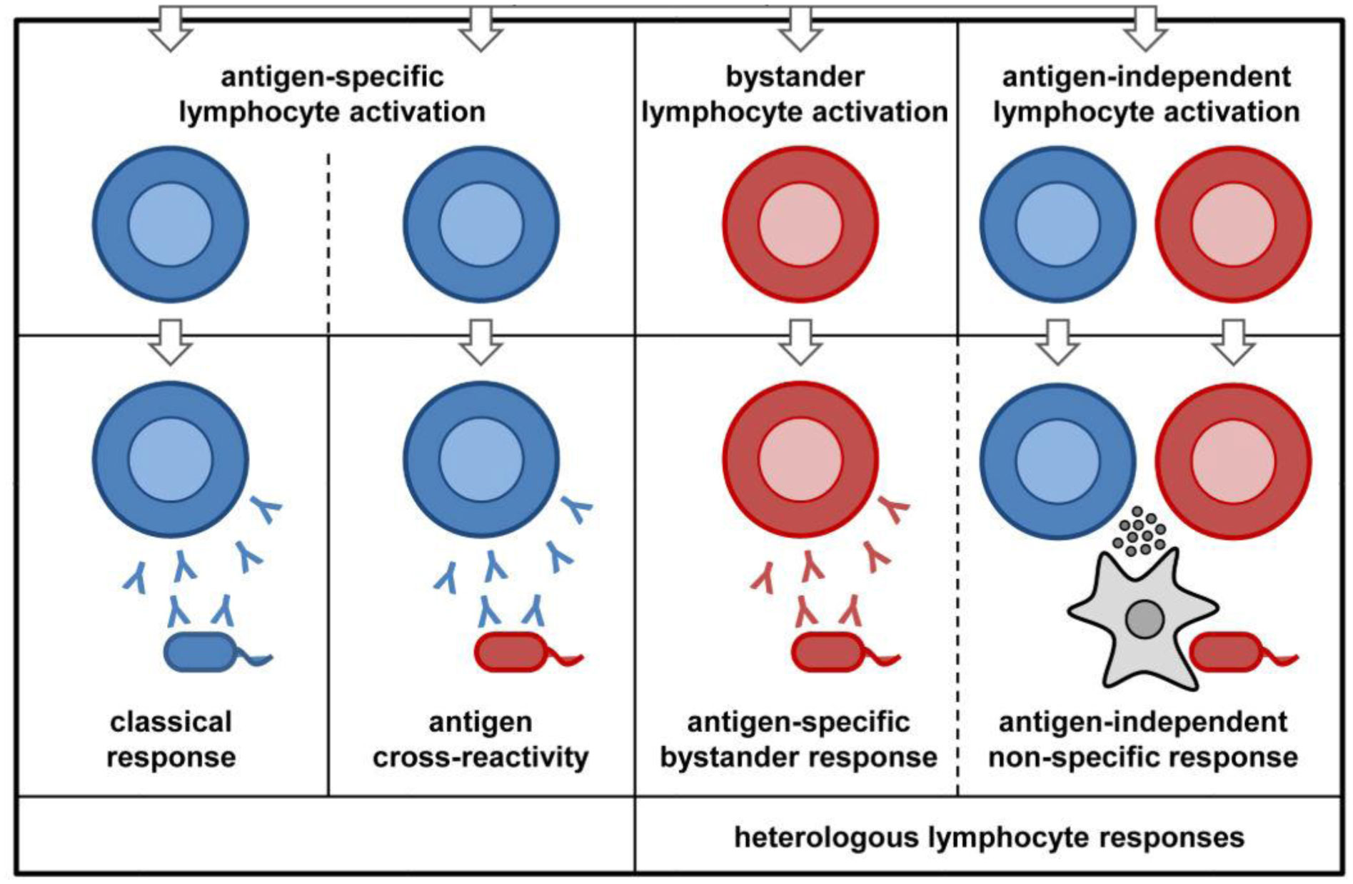
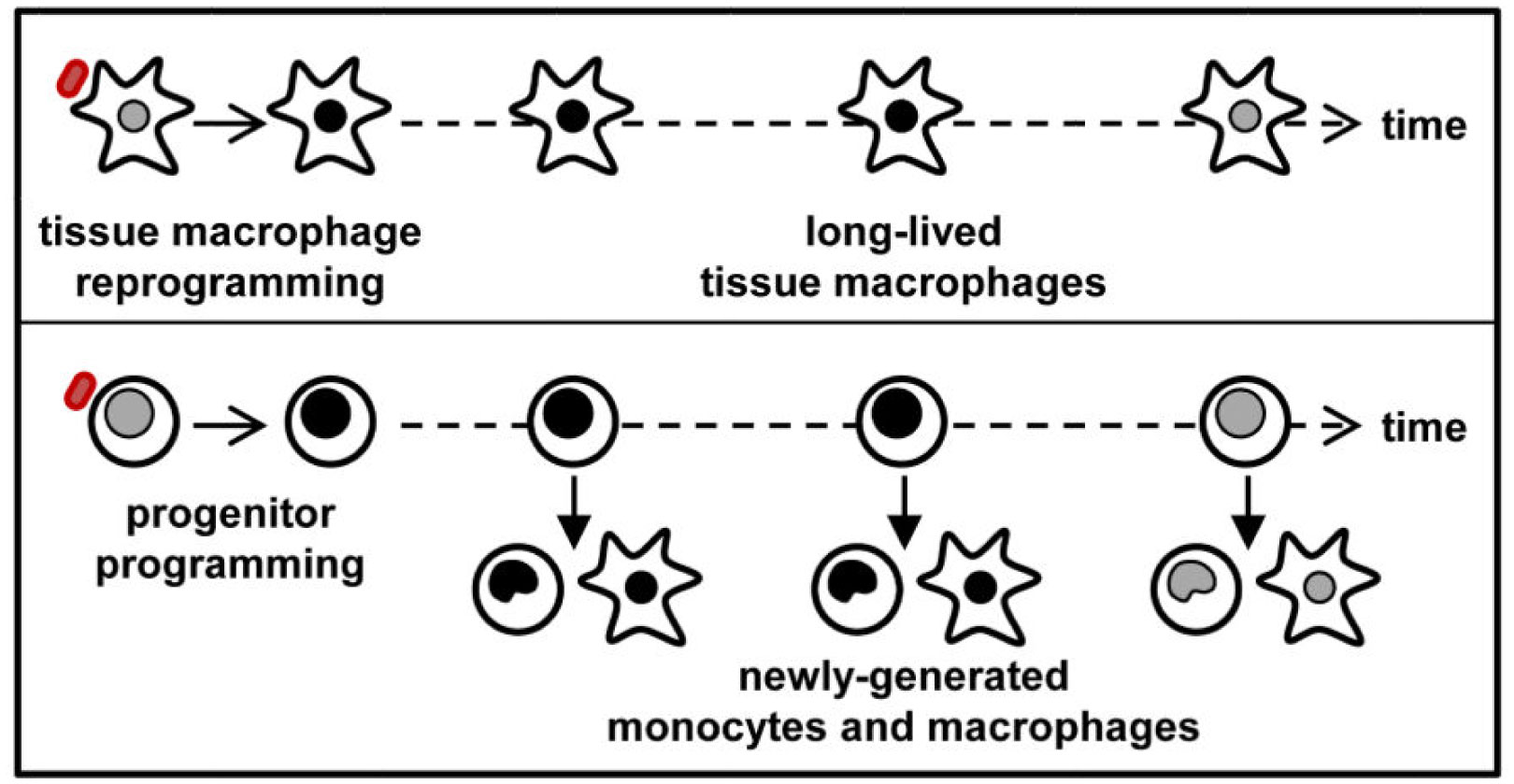
Several epidemiological studies have established that BCG does reduce all-cause mortality in infants, and also the time of vaccination influences this effect significantly. This effect has been attributed to the protective effect of the vaccine in preventing unrelated viral infections during the neonatal period. Some of such viral infections that have been investigated include: herpes simplex virus (HSV), human Papilloma virus (HPV), yellow fever virus (YFV), respiratory syncytial virus (RSV) and influenza virus type A (H1N1). These effects are thought to be mediated via induction of innate immune memory as well as heterologous lymphocytic activation. While epidemiological studies have suggested a correlation, the potential protection of the BCG vaccine against COVID-19 transmission and mortality rates is currently unclear. Ongoing clinical trials and further research may shed more light on the subject in the future.
BCG is a multifaceted vaccine, with many numerous potential applications to vaccination strategies being employed for current and future viral infections. There however is a need for further studies into the immunologic mechanisms behind these non-specific effects, for these potentials to become reality, as we usher in the beginning of the second century since the vaccine's discovery.
Citation: Oluwafolajimi A. Adesanya, Christabel I. Uche-Orji, Yeshua A. Adedeji, John I. Joshua, Adeniyi A. Adesola, Chibuike J. Chukwudike. Bacillus Calmette-Guerin (BCG): the adroit vaccine[J]. AIMS Microbiology, 2021, 7(1): 96-113. doi: 10.3934/microbiol.2021007
The Bacillus Calmette-Guerin (BCG) vaccine has been in use for 99 years, and is regarded as one of the oldest human vaccines known today. It is recommended primarily due to its effect in preventing the most severe forms of tuberculosis, including disseminated tuberculosis and meningeal tuberculosis in children; however, its efficacy in preventing pulmonary tuberculosis and TB reactivation in adults has been questioned. Several studies however have found that asides from its role in tuberculosis prevention, the BCG vaccine also has protective effects against a host of other viral infections in humans, an effect which has been termed: heterologous, non-specific or off-target.
As we approach 100 years since the discovery of the BCG vaccine, we review the evidence of the non-specific protection offered by the vaccine against viral infections, discuss the possible mechanisms of action of these effects, highlight the implications these effects could have on vaccinology and summarize the recent epidemiological correlation between the vaccine and the on-going COVID-19 pandemic.
Several epidemiological studies have established that BCG does reduce all-cause mortality in infants, and also the time of vaccination influences this effect significantly. This effect has been attributed to the protective effect of the vaccine in preventing unrelated viral infections during the neonatal period. Some of such viral infections that have been investigated include: herpes simplex virus (HSV), human Papilloma virus (HPV), yellow fever virus (YFV), respiratory syncytial virus (RSV) and influenza virus type A (H1N1). These effects are thought to be mediated via induction of innate immune memory as well as heterologous lymphocytic activation. While epidemiological studies have suggested a correlation, the potential protection of the BCG vaccine against COVID-19 transmission and mortality rates is currently unclear. Ongoing clinical trials and further research may shed more light on the subject in the future.
BCG is a multifaceted vaccine, with many numerous potential applications to vaccination strategies being employed for current and future viral infections. There however is a need for further studies into the immunologic mechanisms behind these non-specific effects, for these potentials to become reality, as we usher in the beginning of the second century since the vaccine's discovery.

| [1] | Luca S, Mihaescu T (2013) History of BCG vaccine. Maedica (Buchar) 8: 53-58. |
| [2] |
Benévolo-de-Andrade TC, Monteiro-Maia R, Cosgrove C, et al. (2005) BCG Moreau Rio de Janeiro-An oral vaccine against tuberculosis-review. Mem Inst Oswaldo Cruz 100: 459-465. doi: 10.1590/S0074-02762005000500002

|
| [3] | Dagg B, Hockley J, Rigsby P, et al. (2014) The establishment of sub-strain specific WHO Reference Reagents for BCG vaccine 32: 6390-6395. |
| [4] |
Comstock G (1994) The International tuberculosis campaign: a pioneering venture in mass vaccination and research. Clin Infect Dis 19: 528-540. doi: 10.1093/clinids/19.3.528
|
| [5] |
Zwerling A, Behr MA, Verma A, et al. (2011) The BCG World Atlas: A database of global BCG vaccination policies and practices. PLoS Med 8: e1001012. doi: 10.1371/journal.pmed.1001012
|
| [6] |
Trunz BB, Fine P, Dye C (2006) Effect of BCG vaccination on childhood tuberculous meningitis and miliary tuberculosis worldwide: a meta-analysis and assessment of cost-effectiveness. Lancet 367: 1173-1180. doi: 10.1016/S0140-6736(06)68507-3
|
| [7] | Awasthi S, Moin S (1999) Effectiveness of BCG vaccination against tuberculous meningitis. Indian Pediatr 36: 455-460. |
| [8] |
Mangtani P, Abubakar I, Ariti C, et al. (2013) Protection by BCG vaccine against Tuberculosis: a systematic review of randomized controlled trials. Clin Infect Dis 58: 470-80. doi: 10.1093/cid/cit790
|
| [9] |
Setia MS, Steinmaus C, Ho CS, et al. (2006) The role of BCG in prevention of leprosy: A meta-analysis. Lancet Infect Dis 6: 162-170. doi: 10.1016/S1473-3099(06)70412-1
|
| [10] |
Shann F (2013) Nonspecific effects of vaccines and the reduction of mortality in children. Clin Ther 35: 109-114. doi: 10.1016/j.clinthera.2013.01.007
|
| [11] |
Shann F (2010) The non-specific effects of vaccines. Arch Dis Child 95: 662-667. doi: 10.1136/adc.2009.157537
|
| [12] |
Kristensen I, Aaby P, Jensen H (2000) Routine vaccinations and child survival: Follow up study in Guinea-Bissau, West Africa. Br Med J 321: 1435-1439. doi: 10.1136/bmj.321.7274.1435
|
| [13] |
Roth A, Gustafson P, Nhaga A, et al. (2005) BCG vaccination scar associated with better childhood survival in Guinea-Bissau. Int J Epidemiol 34: 540-547. doi: 10.1093/ije/dyh392
|
| [14] |
Garly ML, Martins CL, Balé C, et al. (2003) BCG scar and positive tuberculin reaction associated with reduced child mortality in West Africa: A non-specific beneficial effect of BCG? Vaccine 21: 2782-2790. doi: 10.1016/S0264-410X(03)00181-6
|
| [15] |
Biering-Sørensen S, Aaby P, Lund N, et al. (2017) Early BCG-Denmark and neonatal mortality among infants weighing <2500 g: A randomized controlled trial. Clin Infect Dis 65: 1183-1190. doi: 10.1093/cid/cix525
|
| [16] |
Nankabirwa V, Tumwine JK, Mugaba PM, et al. (2015) Child survival and BCG vaccination: A community based prospective cohort study in Uganda. BMC Public Health 15: 175. doi: 10.1186/s12889-015-1497-8
|
| [17] |
Zimmermann P, Finn A, Curtis N (2018) Does BCG vaccination protect against nontuberculous mycobacterial infection? A systematic review and meta-analysis. J Infect Dis 218: 679-687. doi: 10.1093/infdis/jiy207
|
| [18] |
Aaby P, Roth A, Ravn H, et al. (2011) Randomized Trial of BCG vaccination at birth to low-birth-weight children: beneficial nonspecific effects in the neonatal period? J Infect Dis 204: 245-252. doi: 10.1093/infdis/jir240
|
| [19] |
Biering-Sørensen S, Aaby P, Napirna BM, et al. (2012) Small randomized trial among low-birth-weight children receiving bacillus Calmette-Guéerin vaccination at first health center contact. Pediatr Infect Dis J 31: 306-308. doi: 10.1097/INF.0b013e3182458289
|
| [20] |
Stensballe LG, Sørup S, Aaby P, et al. (2017) BCG vaccination at birth and early childhood hospitalisation: A randomised clinical multicentre trial. Arch Dis Child 102: 224-231. doi: 10.1136/archdischild-2016-310760
|
| [21] |
Stensballe LG, Nante E, Jensen IP, et al. (2005) Acute lower respiratory tract infections and respiratory syncytial virus in infants in Guinea-Bissau: A beneficial effect of BCG vaccination for girls: Community based case-control study. Vaccine 23: 1251-1257. doi: 10.1016/j.vaccine.2004.09.006
|
| [22] | Wardhana, Datau E, Sultana A, et al. (2011) The efficacy of Bacillus Calmette-Guérin vaccinations for the prevention of acute upper respiratory tract infection in the elderly. Acta Med Indones 43: 185-190. |
| [23] |
Ohrui T, Nakayama K, Fukushima T, et al. (2005) Prevention of elderly pneumonia by pneumococcal, influenza and BCG vaccinations. Japanese J Geriatr 42: 34-36. doi: 10.3143/geriatrics.42.34
|
| [24] |
Salem A, Nofal A, Hosny D (2013) Treatment of common and plane warts in children with topical viable bacillus calmette-guerin. Pediatr Dermatol 30: 60-63. doi: 10.1111/j.1525-1470.2012.01848.x
|
| [25] |
Podder I, Bhattacharya S, Mishra V, et al. (2017) Immunotherapy in viral warts with intradermal Bacillus Calmette-Guerin vaccine versus intradermal tuberculin purified protein derivative: A double-blind, randomized controlled trial comparing effectiveness and safety in a tertiary care center in Eastern India. Indian J Dermatol Venereol Leprol 83: 411. doi: 10.4103/0378-6323.188651
|
| [26] |
Daulatabad D, Pandhi D, Singal A (2016) BCG vaccine for immunotherapy in warts: is it really safe in a tuberculosis endemic area? Dermatol Ther 29: 168-172. doi: 10.1111/dth.12336
|
| [27] |
Morales A, Eidinger D, Bruce AW (1976) Intracavitary Bacillus Calmette Guerin in the treatment of superficial bladder tumors. J Urol 116: 180-182. doi: 10.1016/S0022-5347(17)58737-6
|
| [28] | Jackson A, James K (1994) Understanding the most successful immunotherapy for cancer. Immunol 2: 208-215. |
| [29] |
Prescott S, James K, Busuttil A, et al. (1989) HLA—DR Expression by High Grade Superficial Bladder Cancer Treated with BCG. Br J Urol 63: 264-269. doi: 10.1111/j.1464-410X.1989.tb05187.x
|
| [30] |
Jackson AM, Alexandroff AB, McIntyre M, et al. (1994) Induction of ICAM 1 expression on bladder tumours by BCG immunotherapy. J Clin Pathol 47: 309-312. doi: 10.1136/jcp.47.4.309
|
| [31] | Meyer J-P, Persad R (2002) Use of bacille Calmette-Guérin in superficial bladder cancer. Postgrad Med J 78. |
| [32] |
Leentjens J, Kox M, Stokman R, et al. (2015) BCG vaccination enhances the immunogenicity of subsequent influenza vaccination in healthy volunteers: A randomized, placebo-controlled pilot study. J Infect Dis 212: 1930-1938. doi: 10.1093/infdis/jiv332
|
| [33] |
Ritz N, Mui M, Balloch A, et al. (2013) Non-specific effect of Bacille Calmette-Guérin vaccine on the immune response to routine immunisations. Vaccine 31: 3098-3103. doi: 10.1016/j.vaccine.2013.03.059
|
| [34] |
Ota MOC, Vekemans J, Schlegel-Haueter SE, et al. (2002) Influence of Mycobacterium bovis Bacillus Calmette-Guérin on antibody and cytokine responses to human neonatal vaccination. J Immunol 168: 919-925. doi: 10.4049/jimmunol.168.2.919
|
| [35] |
Scheid A, Borriello F, Pietrasanta C, et al. (2018) Adjuvant effect of Bacille Calmette-Guérin on hepatitis B vaccine immunogenicity in the preterm and term newborn. Front Immunol 9: 29. doi: 10.3389/fimmu.2018.00029
|
| [36] |
Arts RJW, Moorlag SJCFM, Novakovic B, et al. (2018) BCG vaccination protects against experimental viral infection in humans through the induction of cytokines associated with trained immunity. Cell Host Microbe 23: 89-100. doi: 10.1016/j.chom.2017.12.010
|
| [37] | FD A, RN U, CL L (1974) Recurrent herpes genitalis. Treatment with Mycobacterium bovis (BCG). Obs Gynecol 43: 797-805. |
| [38] | Hippmann G, Wekkeli M, Rosenkranz A, et al. (1992) Nonspecific immune stimulation with BCG in Herpes simplex recidivans. Follow-up 5 to 10 years after BCG vaccination. Wien Klin Wochenschr 104: 200-204. |
| [39] |
Ahmed SS, Volkmuth W, Duca J, et al. (2015) Antibodies to influenza nucleoprotein cross-react with human hypocretin receptor 2. Sci Transl Med 7. doi: 10.1126/scitranslmed.aab2354
|
| [40] |
Su LF, Kidd BA, Han A, et al. (2013) Virus-Specific CD4+ Memory-Phenotype T Cells Are Abundant in Unexposed Adults. Immunity 38: 373-383. doi: 10.1016/j.immuni.2012.10.021
|
| [41] |
Bernasconi NL, Traggiai E, Lanzavecchia A (2002) Maintenance of serological memory by polyclonal activation of human memory B cells. Science 298: 2199-2202. doi: 10.1126/science.1076071
|
| [42] |
Kleinnijenhuis J, Quintin J, Preijers F, et al. (2014) Long-lasting effects of bcg vaccination on both heterologous th1/th17 responses and innate trained immunity. J Innate Immun 6: 152-158. doi: 10.1159/000355628
|
| [43] |
Vetskova EK, Muhtarova MN, Avramov TI, et al. (2013) Immunomodulatory effects of BCG in patients with recurrent respiratory papillomatosis. Folia Med 55: 49-54. doi: 10.2478/folmed-2013-0005
|
| [44] |
Mathurin KS, Martens GW, Kornfeld H, et al. (2009) CD4 T-Cell-Mediated Heterologous Immunity between Mycobacteria and Poxviruses. J Virol 83: 3528-39. doi: 10.1128/JVI.02393-08
|
| [45] | Kandasamy R, Voysey M, McQuaid F, et al. (2016) Non-specific immunological effects of selected routine childhood immunisations: Systematic review. BMJ 355. |
| [46] |
Netea MG, Joosten LAB, Latz E, et al. (2016) Trained immunity: A program of innate immune memory in health and disease. Science 352: 427. doi: 10.1126/science.aaf1098
|
| [47] |
Kleinnijenhuis J, Quintin J, Preijers F, et al. (2012) Bacille Calmette-Guérin induces NOD2-dependent nonspecific protection from reinfection via epigenetic reprogramming of monocytes. Proc Natl Acad Sci USA 109: 17537-17542. doi: 10.1073/pnas.1202870109
|
| [48] |
Rathinam VAK, Fitzgerald KA (2010) Inflammasomes and anti-viral immunity. J Clin Immunol 30: 632-637. doi: 10.1007/s10875-010-9431-4
|
| [49] |
Allen IC, Scull MA, Moore CB, et al. (2009) The NLRP3 inflammasome mediates in vivo innate immunity to influenza a virus through recognition of viral RNA. Immunity 30: 556-565. doi: 10.1016/j.immuni.2009.02.005
|
| [50] |
Thomas PG, Dash P, Aldridge JR, et al. (2009) The intracellular sensor NLRP3 mediates key innate and healing responses to influenza a virus via the regulation of Caspase-1. Immunity 30: 566-575. doi: 10.1016/j.immuni.2009.02.006
|
| [51] |
Wu F, Zhao S, Yu B, et al. (2020) A new coronavirus associated with human respiratory disease in China. Nature 579: 265-269. doi: 10.1038/s41586-020-2008-3
|
| [52] | Miller A, Reandelar MJ, Fasciglione K, et al. Correlation between universal BCG vaccination policy and reduced morbidity and mortality for COVID-19: an epidemiological study (2020) . |
| [53] |
Scheid A, Borriello F, Pietrasanta C, et al. (2018) Adjuvant effect of Bacille Calmette-Guérin on hepatitis B vaccine immunogenicity in the preterm and term newborn. Front Immunol 9: 24. doi: 10.3389/fimmu.2018.00029
|
| [54] |
Sato H, Jing C, Isshiki M, et al. (2013) Immunogenicity and safety of the vaccinia virus LC16m8δ vector expressing SIV Gag under a strong or moderate promoter in a recombinant BCG prime-recombinant vaccinia virus boost protocol. Vaccine 31: 3549-3557. doi: 10.1016/j.vaccine.2013.05.071
|
| [55] |
Yazdanian M, Memarnejadian A, Mahdavi M, et al. (2013) Immunization of mice by BCG formulated HCV core protein elicited higher th1-oriented responses compared to pluronic-F127 copolymer. Hepat Mon 13. doi: 10.5812/hepatmon.14178
|
| [56] |
Kim BJ, Kim BR, Kook YH, et al. (2018) Development of a live recombinant BCG expressing human immunodeficiency virus type 1 (HIV-1) gag using a pMyong2 vector system: Potential use as a novel HIV-1 vaccine. Front Immunol 9: 27. doi: 10.3389/fimmu.2018.00027
|
| [57] |
Zhou P, Yang X Lou, Wang XG, et al. (2020) A pneumonia outbreak associated with a new coronavirus of probable bat origin. Nature 579: 270-273. doi: 10.1038/s41586-020-2012-7
|
| [58] |
Adesanya OA, Adewale BA, Ebengho IG, et al. (2020) Current knowledge on the pathogenesis of and therapeutic options against SARS-CoV-2: An extensive review of the available evidence. Int J Pathog Res 4: 16-36. doi: 10.9734/ijpr/2020/v4i230108
|
| [59] | Johns Hopkins COVID-19 Map-Johns Hopkins Coronavirus Resource Center (2020) .Available from: https://coronavirus.jhu.edu/map.html. |
| [60] | Hegarty PK, Service NH, Kamat AM, et al. (2020) BCG vaccination may be protective against Covid-19. medRxiv (March). |
| [61] | Dayal D, Gupta S (2020) Connecting BCG Vaccination and COVID-19: Additional Data. medRxiv (April). |
| [62] | Dolgikh S (2020) Further Evidence of a Possible Correlation between the Severity of Covid-19 and BCG Immunization. J Infect Dis Epidemiol 6. |
| [63] |
Sharma A, Kumar Sharma S, Shi Y, et al. (2020) BCG vaccination policy and preventive chloroquine usage: do they have an impact on COVID-19 pandemic? Cell Death Dis 11: 516. doi: 10.1038/s41419-020-2720-9
|
| [64] |
Ebina-Shibuya R, Horita N, Namkoong H, et al. (2020) National policies for paediatric universal BCG vaccination were associated with decreased mortality due to COVID-19. Respirology 25: 898-899. doi: 10.1111/resp.13885
|
| [65] |
Kinoshita M, Tanaka M (2020) Impact of Routine Infant BCG Vaccination on COVID-19. J Infect 81: 625-633. doi: 10.1016/j.jinf.2020.08.013
|
| [66] |
Klinger D, Blass I, Rappoport N, et al. (2020) Significantly improved COVID-19 outcomes in countries with higher bcg vaccination coverage: A multivariable analysis. Vaccines 8: 1-14. doi: 10.3390/vaccines8030378
|
| [67] |
Weng CH, Saal A, Butt WWW, et al. (2020) Bacillus Calmette-Guérin vaccination and clinical characteristics and outcomes of COVID-19 in Rhode Island, United States: A cohort study. Epidemiol Infect 148: e140. doi: 10.1017/S0950268820001569
|
| [68] | Kirov S (2020) Association Between BCG Policy is Significantly Confounded by Age and is Unlikely to Alter Infection or Mortality Rates. medRxiv (April). |
| [69] | Hensel J, McGrail D, McAndrews K, et al. (2020) Exercising caution in correlating COVID-19 incidence and mortality rates with BCG vaccination policies due to variable rates of SARS CoV-2 testing. medRxiv . |
| [70] | (2020) ClinicalTrials.gov.BCG Vaccination to Protect Healthcare Workers Against COVID-19. National Library of Medicine (U.S.). |
| [71] | (2020) ClinicalTrials.gov.Reducing Health Care Workers Absenteeism in Covid-19 Pandemic Through BCG Vaccine. National Library of Medicine (U.S.). |
| [72] | ClinicalTrials.gov. BCG Vaccine for Health Care Workers as Defense Against COVID 19 (2020) . |
| [73] | (2020) ClinicalTrials.gov.BCG Vaccine in Reducing Morbidity and Mortality in Elderly Individuals in COVID-19 Hotspots. National Library of Medicine (U.S.). |
| [74] | Adesanya O, Ebengho I (2020) Possible Correlation between Bacillus Calmette Guérin (BCG) Vaccination Policy and SARS-Cov-2 Transmission, Morbidity and Mortality Rates: Implications for the African Continent. J Infect Dis Epidemiol 6: 137. |
Figures(2) / Tables(2)

Oluwafolajimi A. Adesanya, Christabel I. Uche-Orji, Yeshua A. Adedeji, John I. Joshua, Adeniyi A. Adesola, Chibuike J. Chukwudike. Bacillus Calmette-Guerin (BCG): the adroit vaccine[J]. AIMS Microbiology, 2021, 7(1): 96-113. doi: 10.3934/microbiol.2021007


 DownLoad: