sEMG-based Sarcopenia risk classification using empirical mode decomposition and machine learning algorithms

Konki Sravan Kumar; Daehyun Lee; Ankhzaya Jamsrandoj; Necla Nisa Soylu; Dawoon Jung; Jinwook Kim; Kyung Ryoul Mun; Konki Sravan Kumar; Daehyun Lee; Ankhzaya Jamsrandoj; Necla Nisa Soylu; Dawoon Jung; Jinwook Kim; Kyung Ryoul Mun

doi:10.3934/mbe.2024129

Mathematical Biosciences and Engineering

2024, Volume 21, Issue 2: 2901-2921. doi: 10.3934/mbe.2024129

Previous Article Next Article

Research article Special Issues

sEMG-based Sarcopenia risk classification using empirical mode decomposition and machine learning algorithms

1.
Center for Artificial Intelligence, Korea Institute of Science and Technology, Seoul, Korea
2.
KHU-KIST Department of Converging Science and Technology, Graduate School, Kyung Hee University, Seoul, Korea
3.
Department of Human Computer Interface and Robotics Engineering, University of Science and Technology, Daejeon, Korea
4.
Department of Computer Science, Ozyegin University, Istanbul, Turkey

Received: 29 November 2023 Revised: 28 December 2023 Accepted: 03 January 2024 Published: 25 January 2024

Early detection of the risk of sarcopenia at younger ages is crucial for implementing preventive strategies, fostering healthy muscle development, and minimizing the negative impact of sarcopenia on health and aging. In this study, we propose a novel sarcopenia risk detection technique that combines surface electromyography (sEMG) signals and empirical mode decomposition (EMD) with machine learning algorithms. First, we recorded and preprocessed sEMG data from both healthy and at-risk individuals during various physical activities, including normal walking, fast walking, performing a standard squat, and performing a wide squat. Next, electromyography (EMG) features were extracted from a normalized EMG and its intrinsic mode functions (IMFs) were obtained through EMD. Subsequently, a minimum redundancy maximum relevance (mRMR) feature selection method was employed to identify the most influential subset of features. Finally, the performances of state-of-the-art machine learning (ML) classifiers were evaluated using a leave-one-subject-out cross-validation technique, and the effectiveness of the classifiers for sarcopenia risk classification was assessed through various performance metrics. The proposed method shows a high accuracy, with accuracy rates of 0.88 for normal walking, 0.89 for fast walking, 0.81 for a standard squat, and 0.80 for a wide squat, providing reliable identification of sarcopenia risk during physical activities. Beyond early sarcopenia risk detection, this sEMG-EMD-ML system offers practical values for assessing muscle function, muscle health monitoring, and managing muscle quality for an improved daily life and well-being.
- sEMG,
- empirical mode decomposition,
- feature selection,
- sarcopenia risk,
- machine learning
Citation: Konki Sravan Kumar, Daehyun Lee, Ankhzaya Jamsrandoj, Necla Nisa Soylu, Dawoon Jung, Jinwook Kim, Kyung Ryoul Mun. sEMG-based Sarcopenia risk classification using empirical mode decomposition and machine learning algorithms[J]. Mathematical Biosciences and Engineering, 2024, 21(2): 2901-2921. doi: 10.3934/mbe.2024129

Related Papers:

Abstract

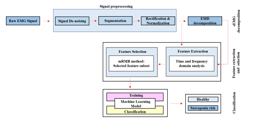
Early detection of the risk of sarcopenia at younger ages is crucial for implementing preventive strategies, fostering healthy muscle development, and minimizing the negative impact of sarcopenia on health and aging. In this study, we propose a novel sarcopenia risk detection technique that combines surface electromyography (sEMG) signals and empirical mode decomposition (EMD) with machine learning algorithms. First, we recorded and preprocessed sEMG data from both healthy and at-risk individuals during various physical activities, including normal walking, fast walking, performing a standard squat, and performing a wide squat. Next, electromyography (EMG) features were extracted from a normalized EMG and its intrinsic mode functions (IMFs) were obtained through EMD. Subsequently, a minimum redundancy maximum relevance (mRMR) feature selection method was employed to identify the most influential subset of features. Finally, the performances of state-of-the-art machine learning (ML) classifiers were evaluated using a leave-one-subject-out cross-validation technique, and the effectiveness of the classifiers for sarcopenia risk classification was assessed through various performance metrics. The proposed method shows a high accuracy, with accuracy rates of 0.88 for normal walking, 0.89 for fast walking, 0.81 for a standard squat, and 0.80 for a wide squat, providing reliable identification of sarcopenia risk during physical activities. Beyond early sarcopenia risk detection, this sEMG-EMD-ML system offers practical values for assessing muscle function, muscle health monitoring, and managing muscle quality for an improved daily life and well-being.

References

[1]	A. Cruz-Jentoft, G. Bahat, J. Bauer, Y. Boirie, O. Bruyère, T. Cederholm, et al., Sarcopenia: Revised European consensus on definition and diagnosis, Age Ag., 48 (2019), 16–31. https://doi.org/10.1093/ageing/afy169 doi: 10.1093/ageing/afy169
[2]	R. A. Fielding, B. Vellas, W. J. Evans, S. Bhasin, J. E. Morley, A. B. Newman, et al., Sarcopenia: An undiagnosed condition in older adults. Current consensus Definition: Prevalence, etiology, and consequences. International Working Group on Sarcopenia, J. Am. Med. Dir. Assoc., 12 (2011), 249–256. https://doi.org/10.1016/j.jamda.2011.01.003 doi: 10.1016/j.jamda.2011.01.003
[3]	I. Janssen, Evolution of sarcopenia research, Appl. Physiol. Nutr. Metab., 35 (2010), 707–712. https://doi.org/10.1139/h10-067 doi: 10.1139/h10-067
[4]	A. Dawson, E. Dennison, Measuring the musculoskeletal aging phenotype, Maturitas, 93 (2016), 13–17. https://doi.org/10.1016/j.maturitas.2016.04.014 doi: 10.1016/j.maturitas.2016.04.014
[5]	C. Beaudart, R. Rizzoli, O. Bruyère, J. Y. Reginster, E. Biver, Sarcopenia: Burden and challenges for public health, Arch. Public Health, 72 (2014). https://doi.org/10.1186/2049-3258-72-45 doi: 10.1186/2049-3258-72-45
[6]	C. Beaudart, E. McCloskey, O. Bruyère, M. Cesari, Y. Rolland, R. Rizzoli, et al., Sarcopenia in daily practice: Assessment and management, BMC Geriatr., 16 (2016). https://doi.org/10.1186/s12877-016-0349-4 doi: 10.1186/s12877-016-0349-4
[7]	M. Cho, S. Lee, S. Song, A review of Sarcopenia Pathophysiology, diagnosis, treatment and future direction, J. Korean Med. Sci, 37 (2022). https://doi.org/10.3346/jkms.2022.37.e146 doi: 10.3346/jkms.2022.37.e146
[8]	D. Albano, C. Messina, J. Vitale, L. M. Sconfienza, Imaging of sarcopenia: Old evidence and new insights, Eur. Radiol., 30 (2020), 2199–2208. https://doi.org/10.1007/s00330-019-06573-2 doi: 10.1007/s00330-019-06573-2
[9]	G. Guglielmi, F. Ponti, M. Agostini, M. Amadori, G. Battista, A. Bazzocchi, The role of DXA in sarcopenia, Ag. Clin. Exp. Res., 28 (2016), 1047–1060. https://doi.org/10.1007/s40520-016-0589-3 doi: 10.1007/s40520-016-0589-3
[10]	P. Tandon, M. Mourtzakis, G. Low, L. Zenith, M. Ney, M. Carbonneau, et al., Comparing the variability between measurements for sarcopenia using magnetic resonance imaging and computed tomography imaging, Am. J. Transplant., 16 (2016), 2766–2767. https://doi.org/10.1111/ajt.13832 doi: 10.1111/ajt.13832
[11]	K. Feng, J. Ji, Q. Ni, A novel gear fatigue monitoring indicator and its application to remaining useful life prediction for spur gear in intelligent manufacturing systems, Int. J. Fatigue, 168 (2023), 107459. https://doi.org/10.1016/j.ijfatigue.2022.107459 doi: 10.1016/j.ijfatigue.2022.107459
[12]	K. Feng, J. Ji, K. Wang, D. Wei, C Zhou, Q Ni, A novel order spectrum-based Vold-Kalman filter bandwidth selection scheme for fault diagnosis of gearbox in offshore wind turbines, Ocean Eng., 266 (2022), 112920. https://doi.org/10.1016/j.oceaneng.2022.112920 doi: 10.1016/j.oceaneng.2022.112920
[13]	K. Feng, J. Ji, Q. Ni, Y Li, W Mao, L Liu, A novel vibration-based prognostic scheme for gear health management in surface wear progression of the intelligent manufacturing system, Wear, 522 (2023), 204697. https://doi.org/10.1016/j.wear.2023.204697 doi: 10.1016/j.wear.2023.204697
[14]	S. Zhao, J. Liu, Z. Gong, Y. S. Lei, X. OuYang, C. C. Chan, et al., Wearable physiological monitoring system based on electrocardiography and electromyography for upper limb rehabilitation training, Sensors, 20 (2020), 4861. https://doi.org/10.3390/s20174861 doi: 10.3390/s20174861
[15]	S. Prabu, K. Srinivas, B. K. Rani, R. Sujat, B. D. Parameshachari, Prediction of muscular paralysis disease based on hybrid feature extraction with machine learning technique for COVID-19 and post-COVID-19 patients, Pers. Ubiquit. Comput., 27 (2023), 831–844. https://doi.org/10.1007/s00779-021-01531-6 doi: 10.1007/s00779-021-01531-6
[16]	I. Campanini, C. Disselhorst-Klug, W. Z. Rymer, R. Merletti, Surface EMG in clinical assessment and neurorehabilitation: Barriers limiting its use, Front. Neurol., 11 (2020), 934. https://doi.org/10.3389/fneur.2020.00934 doi: 10.3389/fneur.2020.00934
[17]	M. Al-Ayyad, H. A. Owida, R. De Fazio, B. Al-Naami, P. Visconti, Electromyography monitoring systems in rehabilitation: A review of clinical applications, wearable devices and signal acquisition methodologies, Electronics, 12 (2023), 1520. https://doi.org/10.3390/electronics12071520 doi: 10.3390/electronics12071520
[18]	R. Habenicht, G. Ebenbichler, P. Bonato, S. Ziegelbecker, L. Unterlerchner, P. Mair, et al., Age-specific differences in the time-frequency representation of surface electromyographic data recorded during a submaximal cyclic back extension exercise: a promising biomarker to detect early signs of sarcopenia, J. NeuroEng. Rehabil., 8 (2020). https://doi.org/10.1186/s12984-020-0645-2 doi: 10.1186/s12984-020-0645-2
[19]	A. Leone, G. Rescio, A. Manni, P. Siciliano, A. Caroppo, Comparative analysis of supervised classifiers for the evaluation of sarcopenia using a sEMG-based platform, Sensors, 22 (2022), 2721. https://doi.org/10.3390/s22072721 doi: 10.3390/s22072721
[20]	J. M. Jasiewicz, J. H. Allum, J. W. Middleton, A. Barriskill, P. Condie, B. Purcell, et al., Gait event detection using linear accelerometers or angular velocity transducers in able-bodied and spinal-cord injured individuals, Gait Posture, 24 (2006), 502–509. https://doi.org/10.1016/j.gaitpost.2005.12.017 doi: 10.1016/j.gaitpost.2005.12.017
[21]	M. Halaki, G. Karen, Normalization of EMG signals: To normalize or not to normalize and what to normalize to?, in computational intelligence in electromyography analysis–a perspective on current applications and future challenges (ed Ganesh R. Naik), InTech, (2012). https://doi.org/10.5772/49957
[22]	E. H. Norden, S. Zheng, L. R. Steven, M. C. Wu, H. H. Shih, Q. N. Zheng, et al., The empirical mode decomposition and the hilbert spectrum for nonlinear and non-stationary time series analysis, in Proceedings: Mathematical, Physical and Engineering Sciences, 454 (1998), 903–995. https://doi.org/10.1098/rspa.1998.0193
[23]	J. Too, A. R. Abdullah, N. M. Saad, Classification of Hand Movements based on Discrete Wavelet Transform and Enhanced Feature Extraction, Int. J. Adv. Comput. Sci. Appl., 10 (2019). https://doi.org/10.14569/ijacsa.2019.0100612 doi: 10.14569/ijacsa.2019.0100612
[24]	S. A. Christopher, I. MdRasedul, A comprehensive study on EMG feature extraction and classifiers, J. Biomed. Eng. Biosci., 1 (2018). https://doi.org/10.32474/oajbeb.2018.01.000104 doi: 10.32474/oajbeb.2018.01.000104
[25]	P. Qin, X. Shi, Evaluation of feature extraction and classification for lower limb motion based on SEMG signal, Entropy, 22 (2020), 852. https://doi.org/10.3390/e22080852 doi: 10.3390/e22080852
[26]	C. Ding, H. Peng, Minimum redundancy feature selection from microarray gene expression data, J. Bioinform. Comput. Biol., 3 (2015), 185–205. https://doi.org/10.1142/s0219720005001004 doi: 10.1142/s0219720005001004
[27]	T. M. Cover, P. D. Hart, Nearest neighbor pattern classification, IEEE Trans. Inf. Theory, 13 (1967), 21–27. https://doi.org/10.1109/tit.1967.1053964 doi: 10.1109/tit.1967.1053964
[28]	M. Hall, A decision Tree-Based attribute weighting filter for naive bayes, In Springer eBooks, 2007, 59–70. https://doi.org/10.1007/978-1-84628-663-6_5 doi: 10.1007/978-1-84628-663-6_5
[29]	T. K. Ho, Random decision forests, Proceedings of 3rd International Conference on Document Analysis and Recognition, 1 (1995), 278-282. doi: 10.1109/ICDAR.1995.598994 doi: 10.1109/ICDAR.1995.598994
[30]	T. Chen, C. Guestrin, XGBoost: A scalable tree boosting system, in Proceedings of the 22nd ACM SIGKDD International Conference on Knowledge Discovery and Data Mining, 2016,785–794. https://doi.org/10.1145/2939672.2939785
[31]	F. Murtagh, Multilayer perceptrons for classification and regression, Neurocomputing, 2 (1991), 183–197. https://doi.org/10.1016/0925-2312(91)90023-5 doi: 10.1016/0925-2312(91)90023-5

Reader Comments

Your name:*

Email:*
© 2024 the Author(s), licensee AIMS Press. This is an open access article distributed under the terms of the Creative Commons Attribution License (http://creativecommons.org/licenses/by/4.0)